How to Analyse the USGS Quaternary Fault Database in Python

On this page

Problem statement

Earthquakes happen on faults, and the faults that matter for hazard are the ones that have moved recently in geological terms. The USGS Quaternary Fault and Fold Database records every fault in the United States known to have moved in the last 1.6 million years, with its age of most recent movement, slip rate, sense of slip and mapping quality, as a national GIS layer of more than 100,000 traces. Using it means getting through a shapefile with categorical attributes written as text, measuring lengths and distances in a projected coordinate system, and choosing which faults count for a question.

This page reads the database for California, measures fault length by slip rate and age, finds the distance from five cities to the nearest fast-slipping and historically active faults, and lists the faults closest to the epicentre of the 2019 Ridgecrest earthquake.

Quick answer

Read the shapefile from the zip, keep California, project to California Albers (EPSG:3310) and sum lengths by class:

ca["km"] = ca.length / 1000
print(f"California: {len(ca):,} traces of {ca.fault_id.nunique():,} faults, {ca.km.sum():,.0f} km in total")
print(ca.groupby("slip_rate").km.sum().sort_values(ascending=False).round(0).to_string())

California: 59,491 traces of 541 faults, 41,931 km in total
slip_rate
Unspecified                  14519.0
Between 0.2 and 1.0 mm/yr     7615.0
Greater than 5.0 mm/yr        6834.0
Between 1.0 and 5.0 mm/yr     6821.0
Less than 0.2 mm/yr           1347.0

California's 59,491 traces belong to 541 faults with 41,931 km of mapped length. The largest slip-rate class by length is "Unspecified", 14,519 km. Faults slipping faster than 5 mm a year make up 6,834 km and those at 1 to 5 mm a year another 6,821 km. The classes add up to 37,136 km, because groupby drops the traces whose slip rate is empty.

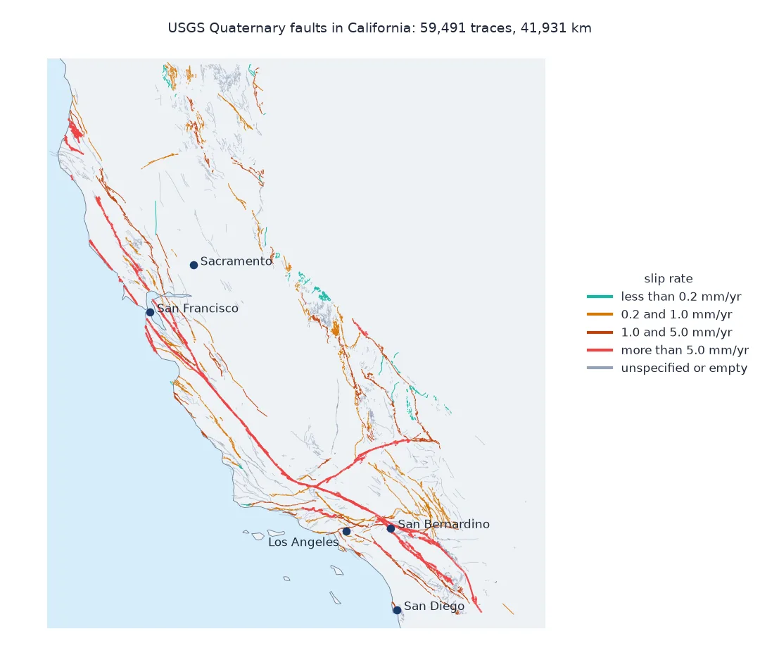
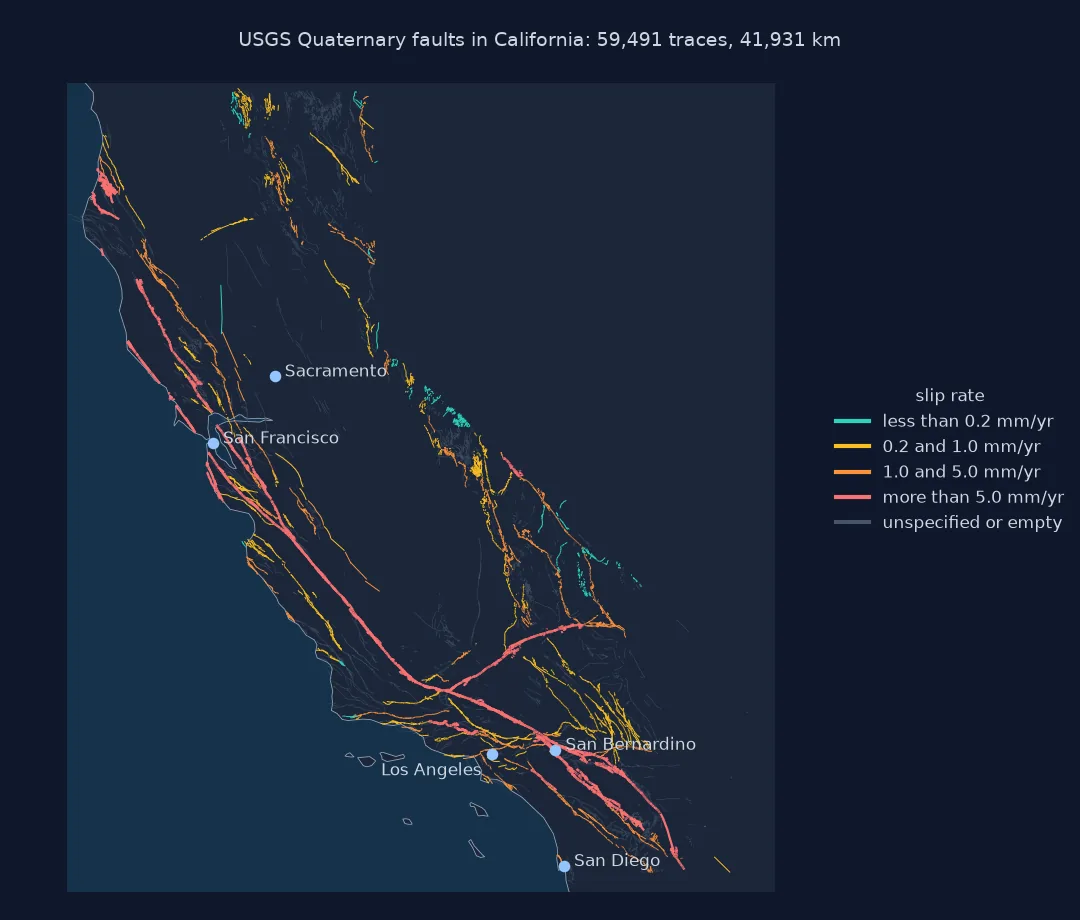
Map of California's mapped Quaternary faults coloured by slip-rate class: the fastest class, more than 5 millimetres a year, traces the San Andreas system, the San Jacinto fault and the east-west Garlock fault in red, slower faults are scattered across the state, and five cities are marked. — California's faults by slip rate.

Check lengths, recent activity, distance from cities

1. Check the lengths

The shapefile is in longitude and latitude, so .length on the original layer is in degrees. The Shape_Leng attribute is in metres, but in which projection? Compare it with lengths measured in EPSG:3310 and in Web Mercator:

deg = qf[qf.Location == "California"].length.sum()
print(f"length in the original CRS: {deg:,.1f} (degrees, meaningless as a distance)")
print(f"Shape_Leng sum: {ca.Shape_Leng.sum() / 1000:,.0f} km; EPSG:3310: {ca.km.sum():,.0f} km; ratio {ca.km.sum() / (ca.Shape_Leng.sum() / 1000):.4f}")
merc = qf[qf.Location == "California"].to_crs(3857).length.sum() / 1000
print(f"Web Mercator (EPSG:3857) length: {merc:,.0f} km; cos(37°) = {np.cos(np.radians(37)):.3f}")

length in the original CRS: 417.6 (degrees, meaningless as a distance)
Shape_Leng sum: 52,480 km; EPSG:3310: 41,931 km; ratio 0.7990
Web Mercator (EPSG:3857) length: 52,480 km; cos(37°) = 0.799

Summed in the original CRS, the length is 417.6, in degrees, which is not a distance. The Shape_Leng attribute sums to 52,480 km, 25% more than the 41,931 km measured in California Albers, and exactly the length in Web Mercator. Web Mercator stretches distances by 1/cos(latitude), and cos(37°) is 0.799, the ratio between the two. The attribute is a Mercator length: do not use it for fault lengths.

2. Recently active faults

The age field gives the time of most recent movement. "Historic" means surface rupture in the last 150 years or so, "latest Quaternary" in the last 15,000 years. Summarise length by age and by sense of slip:

print(ca.groupby("age").km.sum().sort_values(ascending=False).round(0).to_string())
young = ca[ca.age.isin(["historic", "latest Quaternary"])]
print(f"historic or latest Quaternary: {young.km.sum():,.0f} km ({young.km.sum() / ca.km.sum():.0%} of the total)")
print(young.groupby("slip_sense").km.sum().sort_values(ascending=False).head(5).round(0).to_string())

age
undifferentiated Quaternary    18411.0
latest Quaternary              10830.0
late Quaternary                 8964.0
historic                        3724.0
middle and late Quaternary         3.0
historic or latest Quaternary: 14,553 km (35% of the total)
slip_sense
Right lateral    8713.0
Normal           2723.0
Left lateral     1015.0
Thrust            824.0
Reverse           422.0

Most of the length, 18,411 km, is only known to have moved sometime in the Quaternary. 10,830 km moved in the last 15,000 years and 3,724 km in historic time: together 14,553 km, 35% of the total. Most of that young length is right-lateral strike-slip, 8,713 km, the motion of the San Andreas system; normal faults make up 2,723 km.

Age of most recent movement.

3. Distance from cities to faults

Distances in EPSG:3310 are in metres. Find each city's nearest fault slipping faster than 5 mm a year and its nearest historically active fault:

fast = ca[ca.slip_rate == "Greater than 5.0 mm/yr"]
hist = ca[ca.age == "historic"]
for name, pt in cities.geometry.items():
    i = fast.distance(pt).idxmin(); j = hist.distance(pt).idxmin()
    print(f"{name:>14}: fastest-class fault {fast.distance(pt).min() / 1000:5.1f} km ({fast.at[i, 'fault_name']}); "
          f"historic {hist.distance(pt).min() / 1000:5.1f} km ({hist.at[j, 'fault_name']})")

   Los Angeles: fastest-class fault  34.5 km (Sierra Madre fault zone); historic  11.9 km (Newport-Inglewood-Rose Canyon fault zone)
 San Francisco: fastest-class fault  13.6 km (San Andreas fault zone); historic  13.7 km (San Andreas fault zone)
     San Diego: fastest-class fault 101.3 km (Elsinore fault zone); historic  81.7 km (Elsinore fault zone)
    Sacramento: fastest-class fault  94.0 km (Rodgers Creek fault); historic  69.5 km (Green Valley fault)
San Bernardino: fastest-class fault   3.1 km (San Jacinto fault); historic  28.1 km (San Andreas fault zone)

San Bernardino is 3.1 km from the San Jacinto fault, which is in the fastest slip class, and San Francisco 13.6 km from the San Andreas fault zone. Downtown Los Angeles is 11.9 km from the Newport-Inglewood–Rose Canyon fault zone, which ruptured in the 1933 Long Beach earthquake, and 34.5 km from the nearest fastest-class fault. San Diego and Sacramento are 70–100 km from both kinds, by this database's classes.

Faults near the 2019 Ridgecrest epicentre

The data used on this page

The USGS Quaternary Fault and Fold Database as a national shapefile, Qfaults_GIS.zip (32 MB), read directly from the zip. City coordinates are approximate city-hall locations; the Ridgecrest epicentre is from the USGS event page.

from pathlib import Path

import geopandas as gpd
import numpy as np
import pandas as pd
import requests
from shapely.geometry import Point

Path("data").mkdir(exist_ok=True)
z = Path("data/Qfaults_GIS.zip")
if not z.exists():
    r = requests.get("https://earthquake.usgs.gov/static/lfs/nshm/qfaults/Qfaults_GIS.zip", timeout=900)
    r.raise_for_status()
    z.write_bytes(r.content)
qf = gpd.read_file(f"zip://{z}!SHP/Qfaults_US_Database.shp")
ca = qf[qf.Location == "California"].to_crs(3310)
cities = gpd.GeoDataFrame(geometry=[Point(-118.2428, 34.0537), Point(-122.4193, 37.7793), Point(-117.1611, 32.7157),
                                    Point(-121.4944, 38.5816), Point(-117.2898, 34.1083)],
                          index=["Los Angeles", "San Francisco", "San Diego", "Sacramento", "San Bernardino"], crs=4326).to_crs(3310)
print(f"{len(qf):,} traces in the national file, CRS {qf.crs}; California {len(ca):,}")
print(f"slip rate classes: {qf.slip_rate.value_counts(dropna=False).to_dict()}")

112,809 traces in the national file, CRS EPSG:4326; California 59,491
slip rate classes: {'Less than 0.2 mm/yr': 44166, 'Between 0.2 and 1.0 mm/yr': 17112, 'Between 1.0 and 5.0 mm/yr': 16667, 'Greater than 5.0 mm/yr': 16224, 'Unspecified': 14076, nan: 3690, 'Insufficient data': 873, '0.2 +/- 0.1 mm/yr': 1}

The national file has 112,809 traces in longitude and latitude (EPSG:4326), 59,491 of them in California. The slip rate classes are text, with a few oddities: 873 traces marked "Insufficient data", 14,076 "Unspecified", 3,690 empty and one written as "0.2 +/- 0.1 mm/yr".

Example 1: faults near the 2019 Ridgecrest epicentre

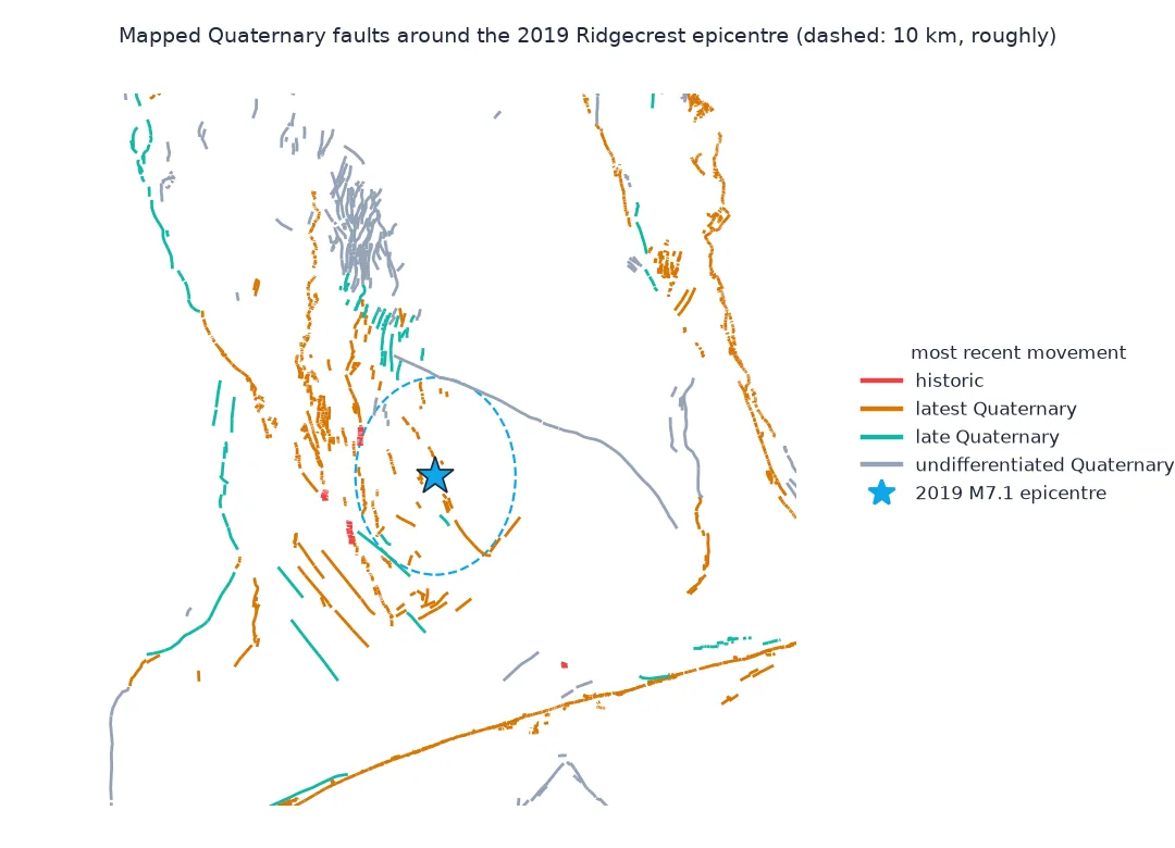
List the distinct faults within 10 km of the M7.1 epicentre, with their age and slip rate:

epi = gpd.GeoSeries([Point(-117.599, 35.770)], crs=4326).to_crs(3310).iloc[0]
near = ca.assign(d_km=ca.distance(epi) / 1000).query("d_km <= 10")
summary = near.groupby("fault_name").agg(traces=("km", "size"), km=("km", "sum"), nearest_km=("d_km", "min"),
                                         age=("age", "first"), slip_rate=("slip_rate", "first")).sort_values("nearest_km")
print(summary.round(1).to_string())

                              traces    km  nearest_km                          age                  slip_rate
fault_name                                                                                                    
Unnamed fault in California       28  30.0         1.7              late Quaternary                        NaN
Little Lake fault zone            42  14.7         5.0            latest Quaternary  Between 1.0 and 5.0 mm/yr
unnamed faults in Coso Range       2   1.6         8.6  undifferentiated Quaternary                        NaN

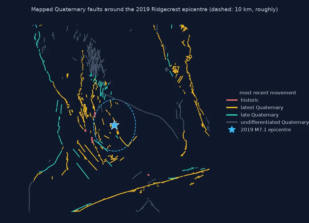
Within 10 km of the 2019 M7.1 epicentre, the database has an unnamed late Quaternary fault 1.7 km away, the Little Lake fault zone at 5.0 km, with a slip rate of 1 to 5 mm a year, and unnamed faults in the Coso Range at 8.6 km. None is marked historic, although the 2019 earthquakes broke the surface along 50 km: the database records what had been mapped and dated, and its California entries were last reviewed in 2017, two years before the earthquakes.

Map of mapped Quaternary faults around the 2019 Ridgecrest epicentre coloured by age of most recent movement, with a dashed circle of about 10 kilometres: latest Quaternary faults run north-south through the area, the Garlock fault crosses the south, and only short historic traces appear, just outside the circle. — Faults near the 2019 epicentre.

How the fault database is compiled

Fault length by slip rate.

The Quaternary Fault and Fold Database is compiled from geological mapping, trenching and dating by the USGS and state geological surveys. Each trace is a mapped segment of a fault at the surface, so one fault appears as many traces, and the same fault can be mapped at different scales in different places. Slip rate and age are given as classes rather than numbers because most faults have not been dated precisely; the classes are what hazard models use to decide how often each fault might rupture.

For hazard, the two attributes work together. A fault slipping more than 5 mm a year, such as the San Andreas, accumulates enough strain for a large earthquake every century or two; a fault slipping less than 0.2 mm a year may go tens of thousands of years between ruptures. A historic or latest Quaternary age says that a fault has ruptured recently enough to be considered active. But the database shows what has been mapped: the 2019 Ridgecrest earthquakes ruptured faults that were only partly mapped before, and blind thrusts that do not reach the surface, such as the one under the 1994 Northridge earthquake, are absent.

Traces against faults, mapping scale and offshore faults

Fault database traps.

Traces, not faults: count fault_id values, not rows, to count faults; sum lengths per fault for fault lengths.
Mapping scale: traces mapped at 1:250,000 are generalised and can be hundreds of metres off; the scale field says which.
Categories as text: slip rate and age are strings, including variants such as "Late Quaternary" and "late Quaternary"; normalise case before grouping.
Offshore faults: offshore California is in a separate layer, ca_offshore, in the same zip.

Internal links

Fixing fault distances computed in degrees — the projection step
How to get seismic hazard curves in Python — what faults feed into
How to map earthquakes against plate boundaries in Python — the global scale

FAQ

Where can I download US fault data?

From the USGS Quaternary Fault and Fold Database, which offers a national shapefile and a web map; this page reads the shapefile directly from the zip.

How do I calculate fault length in Python?

Project the layer to an equal-distance or conformal projected CRS for the region, such as California Albers (EPSG:3310), and use .length, which is then in metres.

What does "latest Quaternary" mean?

Most recent movement within the last 15,000 years; "historic" means a surface rupture within the historical record, roughly the last 150 years in the western US.

Are all active faults in the database?

No: only mapped faults that reach the surface; blind faults and unmapped ones are missing.