How to Get Seismic Hazard Curves in Python

On this page

Problem statement

A seismic hazard curve answers the question building codes are written around: how often, on average, will the ground at this site shake harder than a given level? It is the output of probabilistic seismic hazard analysis, which combines every earthquake source that could affect a site with ground-motion models, and the USGS publishes curves for any point in the conterminous United States through a web service built on its National Seismic Hazard Model. Using the curves means reading annual exceedance rates off a log-log curve, converting rates into the probabilities codes use, and knowing which sources and site conditions are behind them.

This page downloads 2018 national model hazard curves for five US cities, interpolates the ground motions with 10% and 2% chances of exceedance in 50 years, compares peak ground acceleration with a long-period spectral acceleration, splits the hazard into its source types, and shows how much soft soil raises it.

Quick answer

Request the curve for a site, take the total, and interpolate in log-log space at the annual rate you need:

for city in CITIES:
    xs, ys = curve(city, "PGA")
    print(f"{city:>14}: PGA with 10% in 50 yr {at_rate(xs, ys, 1 / 475):.2f} g, with 2% in 50 yr {at_rate(xs, ys, 1 / 2475):.2f} g")

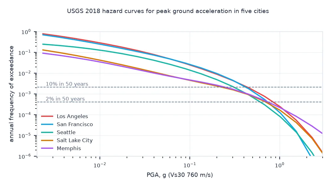
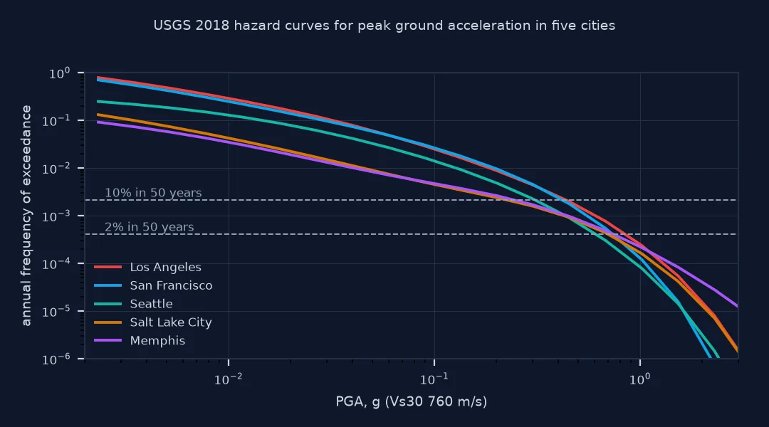
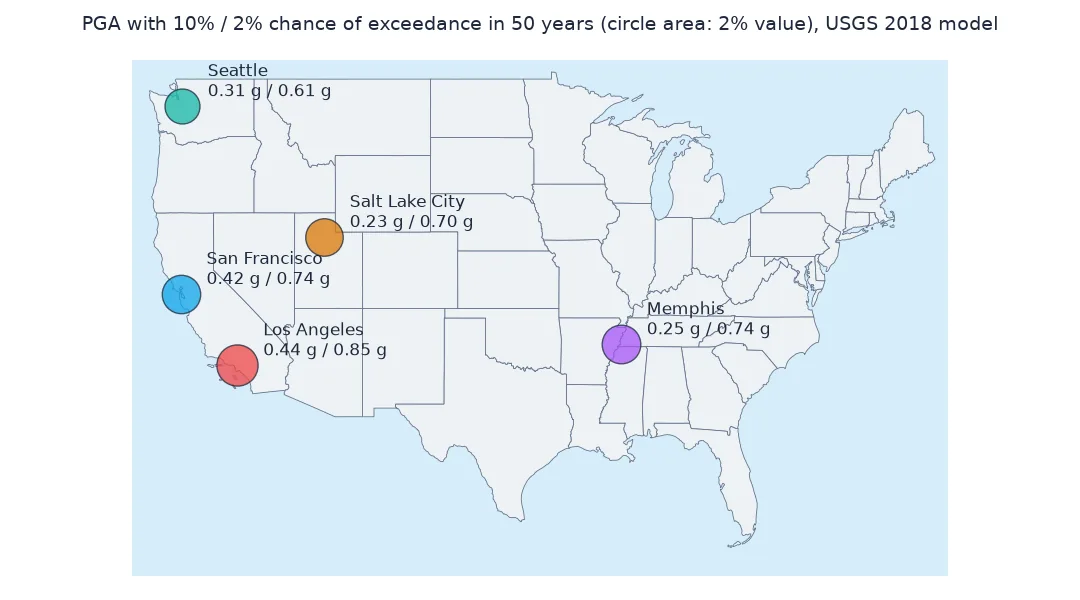
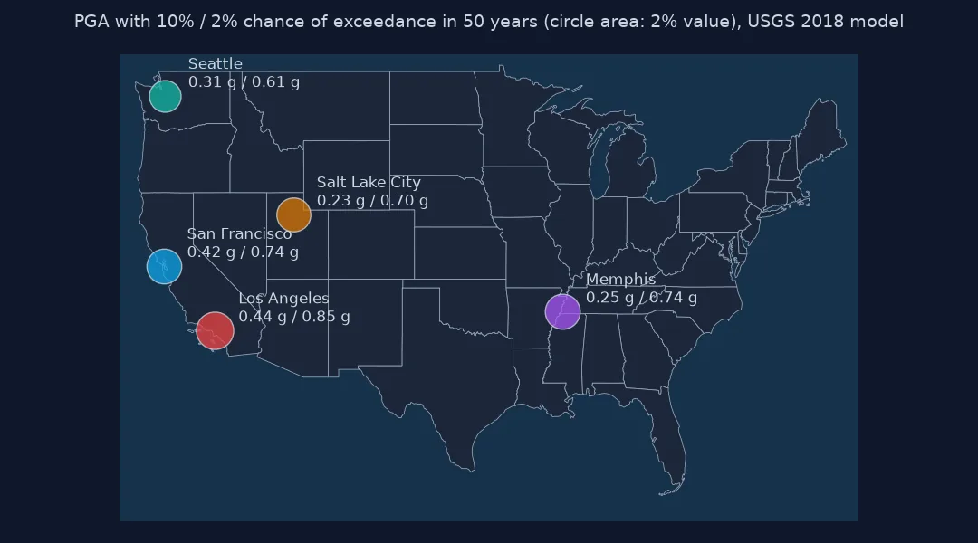
   Los Angeles: PGA with 10% in 50 yr 0.44 g, with 2% in 50 yr 0.85 g
 San Francisco: PGA with 10% in 50 yr 0.42 g, with 2% in 50 yr 0.74 g
       Seattle: PGA with 10% in 50 yr 0.31 g, with 2% in 50 yr 0.61 g
Salt Lake City: PGA with 10% in 50 yr 0.23 g, with 2% in 50 yr 0.70 g
       Memphis: PGA with 10% in 50 yr 0.25 g, with 2% in 50 yr 0.74 g

Los Angeles has the highest values, 0.44 g at 10% in 50 years and 0.85 g at 2%. The ordering changes between the two levels: Salt Lake City and Memphis have the lowest 10%-in-50-years values, 0.23 and 0.25 g, but at 2% in 50 years they pass Seattle, at 0.70 and 0.74 g. Their hazard comes from large earthquakes that are rare, so it rises steeply at long return periods.

Log-log chart of 2018 USGS PGA hazard curves for Los Angeles, San Francisco, Seattle, Salt Lake City and Memphis, with dashed lines at the 10 and 2 percent in 50 years rates: the Los Angeles and San Francisco curves are highest at low ground motions, while Salt Lake City and Memphis start lower and fall more slowly, so that Memphis's curve is the highest beyond about 1 g. — Five cities' hazard curves.

Read the curve, the sources behind it, short and long periods

1. Read the curve

Each curve gives ground-motion levels in g and the annual frequency with which they are exceeded. Print a few points of one:

xs, ys = curve("Los Angeles", "PGA")
for x, y in list(zip(xs, ys))[8:16]:
    print(f"PGA > {x:.3f} g: {y:.2e} a year, return period {1 / y:>9,.0f} years, P(50 years) {1 - np.exp(-50 * y):.1%}")

PGA > 0.060 g: 4.90e-02 a year, return period        20 years, P(50 years) 91.4%
PGA > 0.090 g: 2.90e-02 a year, return period        34 years, P(50 years) 76.6%
PGA > 0.134 g: 1.65e-02 a year, return period        61 years, P(50 years) 56.1%
PGA > 0.202 g: 8.73e-03 a year, return period       115 years, P(50 years) 35.4%
PGA > 0.302 g: 4.38e-03 a year, return period       228 years, P(50 years) 19.7%
PGA > 0.454 g: 1.97e-03 a year, return period       508 years, P(50 years) 9.4%
PGA > 0.680 g: 7.62e-04 a year, return period     1,312 years, P(50 years) 3.7%
PGA > 1.020 g: 2.36e-04 a year, return period     4,232 years, P(50 years) 1.2%

In Los Angeles, PGA above 0.06 g is exceeded about once every 20 years, and above 0.45 g once every 508 years, a 9.4% chance in 50 years. Above 1 g the return period is 4,232 years. The curve's points are spaced by factors of about 1.5 in ground motion, which is why the design values above come from interpolation.

2. Which sources drive the hazard

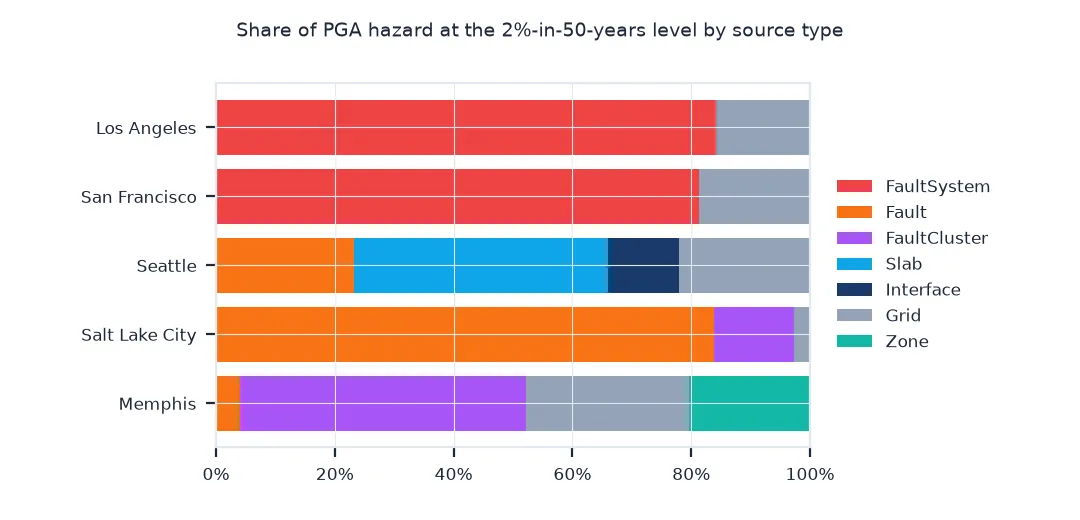
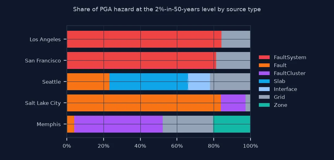
The service splits each curve by source type: individual faults, multi-fault ruptures (FaultSystem), fault clusters such as New Madrid's (FaultCluster), gridded background seismicity (Grid), subduction interface and intraslab sources, and area zones; which appear depends on the site. Take each component's rate at the 2%-in-50-years ground motion:

for city in CITIES:
    comps = components(city, "PGA")
    x2 = at_rate(*curve(city, "PGA"), 1 / 2475)
    share = {k: np.exp(np.interp(np.log(x2), np.log(v[0]), np.log(np.maximum(v[1], 1e-30)))) for k, v in comps.items() if k != "Total"}
    tot = sum(share.values())
    print(f"{city:>14}: " + ", ".join(f"{k} {s / tot:.0%}" for k, s in sorted(share.items(), key=lambda kv: -kv[1]) if s / tot >= 0.01))

   Los Angeles: FaultSystem 84%, Grid 16%
 San Francisco: FaultSystem 81%, Grid 19%
       Seattle: Slab 43%, Fault 23%, Grid 22%, Interface 12%
Salt Lake City: Fault 84%, FaultCluster 13%, Grid 3%
       Memphis: FaultCluster 48%, Grid 27%, Zone 20%, Fault 4%

The sources differ completely between the cities. In Los Angeles and San Francisco, more than 80% of the hazard at the 2%-in-50-years level comes from the fault-system model, ruptures on the dense network of California faults. In Seattle, the largest part, 43%, comes from earthquakes inside the subducting slab, and 12% from the Cascadia interface. Salt Lake City's hazard is 84% individual faults; Memphis's 48% the New Madrid clusters.

Stacked bar chart of the share of PGA hazard at the 2 percent in 50 years level by source type: Los Angeles and San Francisco over 80 percent fault system; Seattle 43 percent slab, 23 percent fault, 22 percent gridded and 12 percent interface; Salt Lake City 84 percent fault; Memphis 48 percent fault cluster, 27 percent gridded and 20 percent zone. — What drives the hazard.

3. Short and long periods

Peak ground acceleration matters for stiff, short buildings; the 1-second spectral acceleration for tall ones. Compare them at the 2%-in-50-years level:

for city in CITIES:
    pga = at_rate(*curve(city, "PGA"), 1 / 2475)
    sa1 = at_rate(*curve(city, "SA1P0"), 1 / 2475)
    print(f"{city:>14}: PGA {pga:.2f} g, SA(1.0 s) {sa1:.2f} g, ratio {sa1 / pga:.2f}")

   Los Angeles: PGA 0.85 g, SA(1.0 s) 0.64 g, ratio 0.75
 San Francisco: PGA 0.74 g, SA(1.0 s) 0.60 g, ratio 0.82
       Seattle: PGA 0.61 g, SA(1.0 s) 0.58 g, ratio 0.96
Salt Lake City: PGA 0.70 g, SA(1.0 s) 0.57 g, ratio 0.81
       Memphis: PGA 0.74 g, SA(1.0 s) 0.33 g, ratio 0.44

The ratio of the 1-second spectral acceleration to PGA tells which buildings the hazard threatens most. It is 0.96 in Seattle, where subduction-zone and intraslab earthquakes contribute most, and 0.44 in Memphis.

Hazard on soft soil

The data used on this page

Hazard curves from the USGS hazard curve web service for the 2018 conterminous US National Seismic Hazard Model, on site class B/C (Vs30 = 760 m/s) and, for one city, on soft soil (Vs30 = 259 m/s). Coordinates are approximate city centres. Each request takes about 20 seconds, so the setup saves the responses.

import json
from pathlib import Path

import numpy as np
import requests

Path("data").mkdir(exist_ok=True)
CITIES = {"Los Angeles": (34.05, -118.25), "San Francisco": (37.78, -122.42), "Seattle": (47.61, -122.33),
          "Salt Lake City": (40.76, -111.89), "Memphis": (35.15, -90.05)}
def response(city, vs30=760):
    lat, lon = CITIES[city]
    p = Path(f"data/nshm2018_{city.replace(' ', '_')}_{vs30}.json")
    if not p.exists():
        r = requests.get(f"https://earthquake.usgs.gov/ws/nshmp/conus-2018/dynamic/hazard/{lon}/{lat}/{vs30}", timeout=300)
        r.raise_for_status()
        p.write_text(r.text)
    return json.loads(p.read_text())["response"]
def components(city, imt, vs30=760):
    c = next(h for h in response(city, vs30)["hazardCurves"] if h["imt"]["value"] == imt)
    return {d["component"]: (np.array(d["values"]["xs"]), np.array(d["values"]["ys"])) for d in c["data"]}
def curve(city, imt, vs30=760):
    return components(city, imt, vs30)["Total"]
def at_rate(xs, ys, rate):
    ok = ys > 0
    return float(np.exp(np.interp(np.log(rate), np.log(ys[ok][::-1]), np.log(xs[ok][::-1]))))
r = response("Los Angeles")
print(f"x axis: {r['metadata']['xlabel']}; y axis: {r['metadata']['ylabel']}")
print(f"intensity measures: {len(r['hazardCurves'])}; points per curve: {len(curve('Los Angeles', 'PGA')[0])}")

x axis: Ground Motion (g); y axis: Annual Frequency of Exceedance
intensity measures: 23; points per curve: 20

Each response holds curves for 23 intensity measures, from PGA and PGV to spectral accelerations at periods from 0.01 to 10 seconds, each as 20 ground-motion levels in g with their annual frequencies of exceedance.

Example 1: soft soil

Site conditions change the hazard. Compare Los Angeles on site class B/C with the same point on soft soil, for PGA and the 1-second spectral acceleration:

for imt in ("PGA", "SA1P0"):
    rock = at_rate(*curve("Los Angeles", imt, 760), 1 / 2475)
    soft = at_rate(*curve("Los Angeles", imt, 259), 1 / 2475)
    print(f"{imt:>6}: Vs30 760 {rock:.2f} g, Vs30 259 {soft:.2f} g, factor {soft / rock:.2f}")

   PGA: Vs30 760 0.85 g, Vs30 259 0.87 g, factor 1.02
 SA1P0: Vs30 760 0.64 g, Vs30 259 1.46 g, factor 2.29

On soft soil the 2%-in-50-years PGA in Los Angeles hardly changes, from 0.85 to 0.87 g, but the 1-second spectral acceleration more than doubles, from 0.64 to 1.46 g. At such strong shaking, soft soils amplify short-period motion little, while long-period motion is amplified strongly.

Soft soil and period.

PSHA sums over every possible earthquake

Map of the conterminous United States with circles at five cities sized by their 2 percent in 50 years PGA and labelled with the 10 and 2 percent values: Seattle 0.31 and 0.61 g, San Francisco 0.42 and 0.74, Los Angeles 0.44 and 0.85, Salt Lake City 0.23 and 0.70, Memphis 0.25 and 0.74. — Design ground motions in five cities.

Probabilistic seismic hazard analysis sums over every possible earthquake: for each source, how often earthquakes of each magnitude occur, where they could be, and the probability that each would shake the site beyond a given level according to a ground-motion model with its scatter. The total annual rate of exceedance at each level makes the hazard curve. Reading it is one interpolation: pick a rate, read the ground motion. Codes choose rates by probability over a building's life: 10% in 50 years is a rate of 1/475 a year, 2% in 50 years 1/2,475.

The components show what drives the hazard, which matters for design. Where it comes from nearby faults, as in California, the controlling earthquakes are close and of moderate to large magnitude; where subduction contributes, as in the Pacific Northwest, they can be distant and very large, with long durations and strong long-period shaking. Site conditions enter through Vs30: the national maps are drawn for a reference site class, and soft soils amplify, more so for long periods and moderate shaking than for very strong shaking, where soils can become nonlinear and amplify less.

Model editions, interpolation and Vs30

Before using a hazard curve.

Model editions: the service offers several editions (2008, 2014, 2018 and newer); values change between them, so record which one.
Interpolation: always interpolate in log-log space; linear interpolation between the curve's points underestimates.
Risk-targeted design values: building codes now use risk-targeted ground motions derived from these curves, not the 2%-in-50-years value directly.
Vs30 choices: the service accepts a fixed set of Vs30 values; for others, use a site-specific study.

Internal links

Seismic hazard explained — what the curve means
How to map seismic hazard in Python — the same idea as a map
Fixing peak ground acceleration values that are 100 times too large — g against percent of g

FAQ

What is a seismic hazard curve?

A curve of ground-motion level against the annual frequency with which it is exceeded at a site, from probabilistic seismic hazard analysis.

How do I get USGS hazard curves in Python?

Request https://earthquake.usgs.gov/ws/nshmp/conus-2018/dynamic/hazard/{longitude}/{latitude}/{vs30} with requests and read response.hazardCurves.

What does 2% in 50 years mean?

A ground motion with a 2% chance of being exceeded at least once in 50 years, equivalent to an annual rate of 1/2,475.

Why is Memphis's hazard so different from Los Angeles's?

Memphis's hazard comes mainly from the New Madrid seismic zone, modelled as clusters of large but infrequent earthquakes, which contribute 48% at the 2%-in-50-years level. Its 10%-in-50-years PGA, 0.25 g, is little more than half of Los Angeles's, but its 2%-in-50-years value, 0.74 g, is close: rare, large earthquakes make its curve flatter.