How to map burn severity with dNBR in Python

On this page

Problem statement

Mapping burn severity needs two cloud-free Sentinel-2 scenes, four bands and one subtraction. The work is in the parts either side: choosing scenes that differ by the fire and not by the season, putting both on the same grid, masking cloud and water, applying an offset measured off unburned ground, and stating which assessment — immediate or a season later — the map represents.

This guide maps the 2024 Park Fire in northern California, from scenes on 2 July and 10 September 2024, and then repeats the calculation with a scene from the following summer to show how much the answer moves.

Quick answer

Read matching bands from a pre- and a post-fire scene onto one grid and difference the normalised burn ratio:

import numpy as np, pystac_client, rasterio
from rasterio.enums import Resampling
from rasterio.transform import from_origin
from rasterio.vrt import WarpedVRT
from rasterio.warp import transform_bounds
from shapely.geometry import box, shape

BBOX = [-122.00, 40.00, -121.74, 40.22]                 # inside the Park Fire perimeter
CRS, RES = "EPSG:32610", 20
left, bottom, right, top = transform_bounds(4326, CRS, *BBOX)
GRID = {"crs": CRS, "transform": from_origin(left, top, RES, RES),
        "width": int((right - left) // RES), "height": int((top - bottom) // RES)}

es = pystac_client.Client.open("https://earth-search.aws.element84.com/v1")

def scene(dates, max_cloud=5):
    aoi = box(*BBOX)
    items = [i for i in es.search(collections=["sentinel-2-c1-l2a"], bbox=BBOX, datetime=dates,
                                  query={"eo:cloud_cover": {"lt": max_cloud}}).item_collection()
             if shape(i.geometry).contains(aoi)]
    return sorted(items, key=lambda i: i.datetime)[0]

def band(item, name):
    with rasterio.open(item.assets[name].href) as src, WarpedVRT(
            src, crs=GRID["crs"], transform=GRID["transform"], width=GRID["width"],
            height=GRID["height"], resampling=Resampling.bilinear) as vrt:
        a = vrt.read(1).astype("float32")
    return np.where(a > 0, a * 0.0001, np.nan)          # scene-classification zeros out

def nbr(item):
    return (band(item, "nir08") - band(item, "swir22")) / (band(item, "nir08") + band(item, "swir22"))

pre, post = scene("2024-07-01/2024-07-10"), scene("2024-09-08/2024-09-15")
dnbr = (nbr(pre) - nbr(post)) * 1000
print(f"pre {pre.id} ({pre.datetime.date()}), post {post.id} ({post.datetime.date()})")
print(f"dNBR median {np.nanmedian(dnbr):.0f}, 95th percentile {np.nanpercentile(dnbr, 95):.0f}")

pre S2A_T10TEK_20240702T185828_L2A (2024-07-02), post S2A_T10TEK_20240910T185948_L2A (2024-09-10)
dNBR median 198, 95th percentile 506

Bands 8A (nir08) and 12 (swir22) are the Sentinel-2 equivalents of the Landsat bands the dNBR thresholds were derived with.

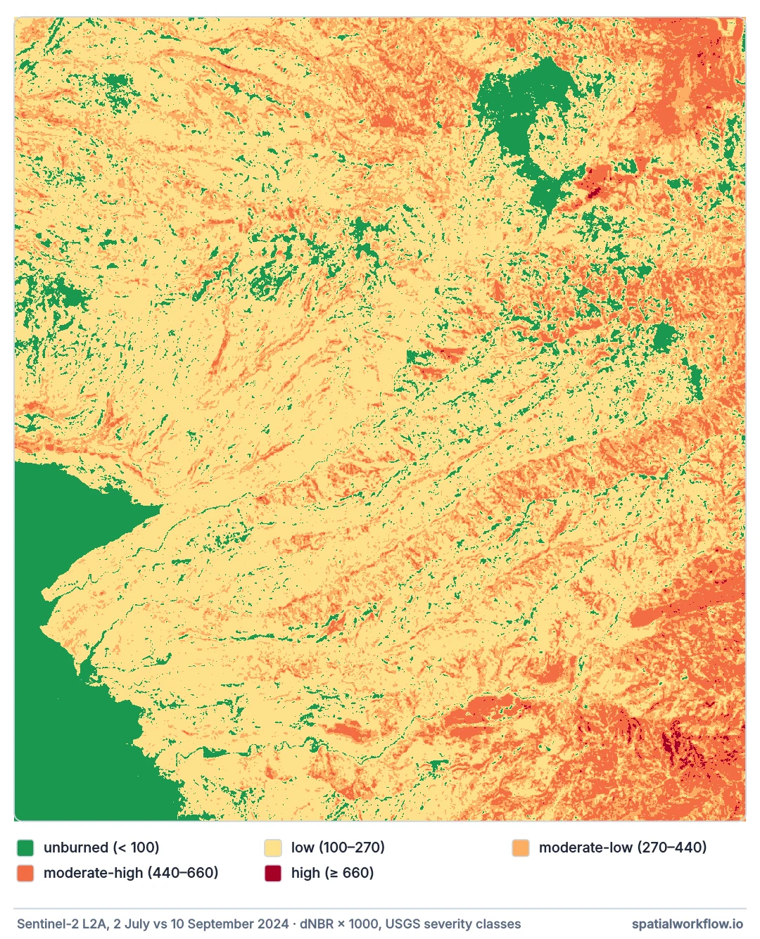
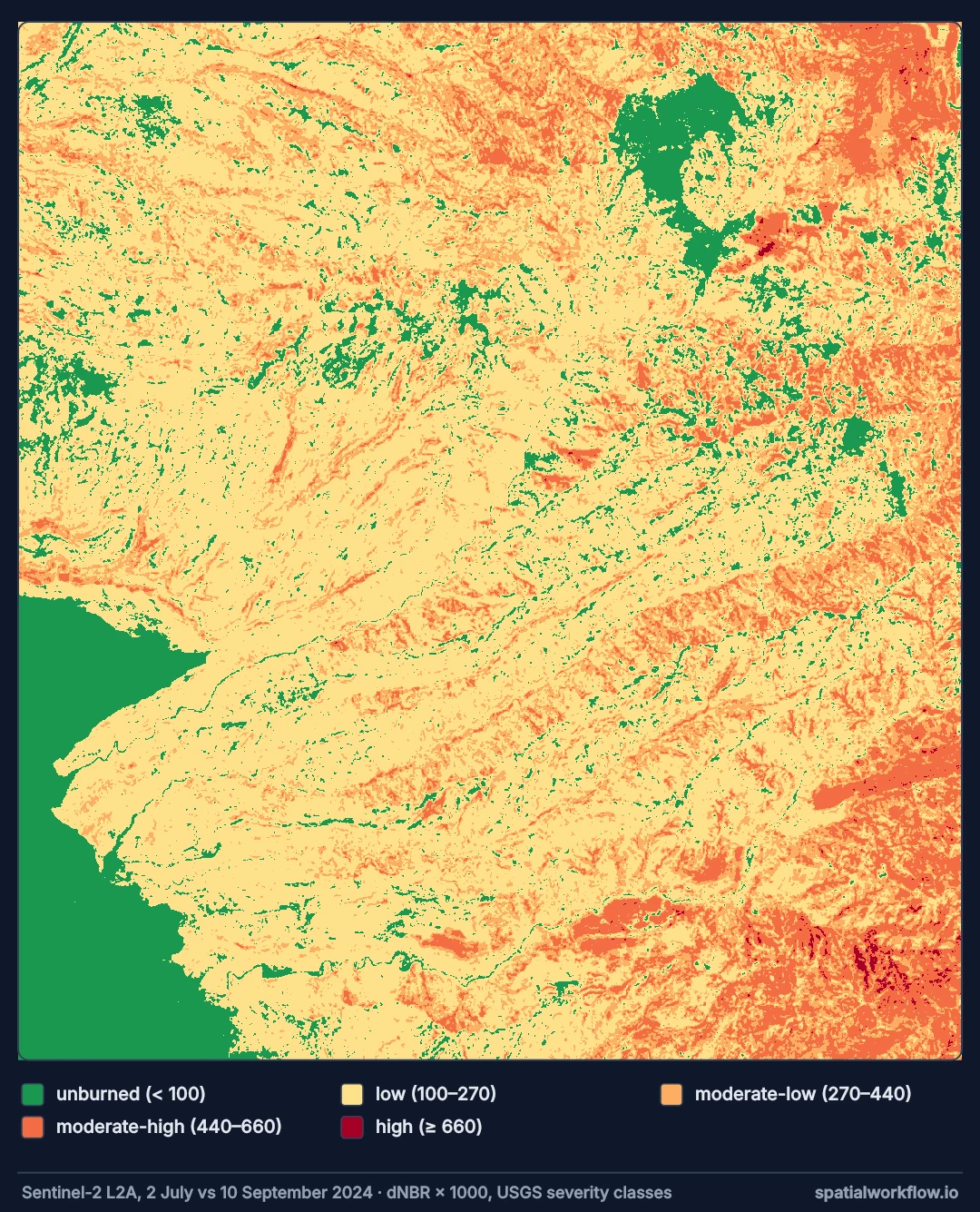
Map of a window inside the 2024 Park Fire classed by burn severity: most of it low severity in pale yellow, moderate and high severity in orange and dark red concentrated in the south-east and north-east, and unburned green at the south-west corner. — The dNBR from the code above, in the USGS severity classes. Most of the window burned at low severity — median dNBR 198 — with the moderate-to-high burns concentrated in the south-east and north-east. The large unburned area in the south-west corner is low ground the fire did not reach.

Seven steps, of which two — scene choice and the offset — decide most of the result.

Matched scenes, one grid, masks, an offset, classes

1. Pick scenes that differ by the fire

Same tile, low cloud, and as close to the same point in the season as the fire allows. Check that the pre-fire scene really predates ignition.

2. Put both on one grid

Read through a warped VRT onto a grid you define, so the two arrays align exactly and the output has a CRS you chose.

3. Mask what is not vegetation

Water, cloud and cloud shadow produce extreme dNBR values. The scene classification band (scl) marks them.

4. Offset-correct

Subtract the median dNBR of unburned ground outside the perimeter. It is usually small, and it is the difference between a map of the fire and a map of the fire plus two months of drying.

5. Classify, and say whose thresholds

The USGS breaks are the default. Print the area in each class so a reader can see how the map is distributed.

6. Write the metadata into the file

Scene IDs, dates, offset, thresholds, CRS. A severity GeoTIFF without them cannot be compared with anyone else's.

The same fire and the same window, assessed two months later and eleven months later.

Masking and classifying Park Fire severity

The data used on this page

Sentinel-2 L2A scenes from the Element 84 Earth Search STAC catalogue (the code picks them), and the 2024 Park Fire perimeter from the WFIGS interagency fire perimeters feature service, saved as park_perimeter.geojson.

import os

import requests

WFIGS = ("https://services3.arcgis.com/T4QMspbfLg3qTGWY/arcgis/rest/services/"
         "WFIGS_Interagency_Perimeters/FeatureServer/0/query")
if not os.path.exists("park_perimeter.geojson"):
    reply = requests.get(WFIGS, params={"where": "poly_IncidentName='PARK' AND attr_POOState='US-CA'",
                                        "outFields": "*", "f": "geojson", "outSR": 4326}, timeout=300)
    reply.raise_for_status()
    open("park_perimeter.geojson", "w").write(reply.text)
print(os.path.getsize("park_perimeter.geojson") > 0)

True

Example 1 — mask cloud, shadow and water with the scene classification

def scl(item):
    with rasterio.open(item.assets["scl"].href) as src, WarpedVRT(
            src, crs=GRID["crs"], transform=GRID["transform"], width=GRID["width"],
            height=GRID["height"], resampling=Resampling.nearest) as vrt:
        return vrt.read(1)

BAD = {0, 1, 3, 6, 8, 9, 10, 11}                         # nodata, saturated, shadow, water, clouds, snow
mask = np.isin(scl(pre), list(BAD)) | np.isin(scl(post), list(BAD))
print(f"masked pixels: {mask.mean():.2%}")
clean = np.where(mask, np.nan, dnbr)
print(f"dNBR median before masking {np.nanmedian(dnbr):.0f}, after {np.nanmedian(clean):.0f}")

masked pixels: 0.00%
dNBR median before masking 198, after 198

Nothing is masked in this pair: both scenes are cloud-free over the window, and the fire is well inland of any water. Run the step anyway — on the one pair where it matters, it decides the whole summary.

Example 2 — offset and classify

import geopandas as gpd
from rasterio.features import geometry_mask

fire = gpd.read_file("park_perimeter.geojson")
fire = fire[fire.poly_GISAcres > 1000].to_crs(GRID["crs"])
inside = geometry_mask(fire.geometry, out_shape=(GRID["height"], GRID["width"]),
                       transform=GRID["transform"], invert=True)

offset = np.nanmedian(clean[~inside])
corrected = clean - offset
CLASSES = [(-100, 99, "unburned"), (99, 269, "low"), (269, 439, "moderate-low"),
           (439, 659, "moderate-high"), (659, 2000, "high")]
print(f"offset from unburned ground: {offset:+.0f} dNBR")
for lo, hi, name in CLASSES:
    m = (corrected >= lo) & (corrected < hi) & inside
    print(f"  {name:14} {np.nansum(m) * RES * RES / 1e6:7.1f} km²")

offset from unburned ground: -9 dNBR
  unburned          31.5 km²
  low              321.7 km²
  moderate-low     112.8 km²
  moderate-high     55.8 km²
  high               1.5 km²

Example 3 — the extended assessment

post_next = scene("2025-07-01/2025-07-20")
dnbr_ext = ((nbr(pre) - nbr(post_next)) * 1000) - offset
print(f"extended post-fire scene: {post_next.id} ({post_next.datetime.date()})")
for lo, hi, name in CLASSES:
    a = np.nansum((corrected >= lo) & (corrected < hi) & inside) * RES * RES / 1e6
    b = np.nansum((dnbr_ext >= lo) & (dnbr_ext < hi) & inside) * RES * RES / 1e6
    print(f"  {name:14} initial {a:7.1f} km²   extended {b:7.1f} km²")

extended post-fire scene: S2B_T10TEK_20250702T190248_L2A (2025-07-02)
  unburned       initial    31.5 km²   extended   339.0 km²
  low            initial   321.7 km²   extended   152.4 km²
  moderate-low   initial   112.8 km²   extended    27.3 km²
  moderate-high  initial    55.8 km²   extended     4.5 km²
  high           initial     1.5 km²   extended     0.0 km²

A year later, two thirds of the window has moved back into the unburned class and the moderate-high area has fallen from 56 km² to 4.5. Nothing about the fire changed; the grass and shrubs came back, and NBR came back with them. Neither map is wrong, and a map that does not say which assessment it is cannot be read at all.

Why the offset and masking are not optional

Why the offset is not optional

Two months apart, unburned vegetation has dried, shadows have moved and the atmosphere has changed. All of that lands in dNBR as a constant-ish shift. Measuring it on ground that did not burn and subtracting it is the cheapest correction in the workflow and the one most often skipped.

Why masking comes before classifying

Water has a very high NBR and burns have a low one, so a lake that dries between scenes produces enormous dNBR. Cloud shadow does the same in reverse. Those pixels then dominate any summary statistic, and they are not fire.

Why initial and extended assessments differ

An initial assessment measures what the fire did: consumed canopy, blackened ground. A year later, grass and shrubs have returned over some of it and the ground is no longer bare, so dNBR falls and area shifts towards the lower classes. Which one to use depends on the question — immediate effects, or persistent change.

Five classes of pixel that produce extreme dNBR without any fire.

Landsat, long fires and smoke

Landsat gives a longer archive; bands 5 and 7 replace 8A and 12.
Fires that burn for weeks need a post-fire scene after containment, not during.
Smoke in the post-fire scene lowers NIR and biases severity upwards.
Sentinel-2 L2A surface reflectance has a scale factor of 10,000 and, in newer processing baselines, an offset too.
Compare with the official product where one exists: MTBS in the US publishes mapped severity for large fires.
RdNBR needs pre-fire NBR in the denominator and has its own thresholds.

Internal links

Burn severity explained — what the index and classes mean
dNBR shows change outside the fire perimeter — the fix guide
How to work with fire perimeter data in Python — the perimeter used here
How to count buildings and people exposed to a hazard zone — severity into exposure
How to mask clouds in Sentinel-2 imagery in Python — the SCL band in detail
Vegetation indices explained — NBR's relatives

FAQ

Which Sentinel-2 bands do I need for dNBR?

Band 8A (nir08) and band 12 (swir22).

How soon after a fire should the post-fire scene be?

For an initial assessment, as soon after containment as cloud allows; for an extended assessment, the next growing season.

What offset should I apply?

The median dNBR of unburned ground outside the perimeter, measured from your own scenes.

Do I have to mask water?

Yes. Water produces extreme NBR values that swamp any summary.

Which thresholds should I use?

The USGS FIREMON breaks are conventional; state them, and check them against imagery.

Why does my burned area differ from the official figure?

Different scenes, thresholds, offset and assessment timing — all four change the answer.