
Choosing a Map Projection for Display: What Web Mercator Distorts
On this page
Problem statement
You plot a choropleth of European countries and Scandinavia dominates the page. You plot a world map of population density and Greenland looks comparable to Africa. You compute area from a plot in EPSG:4326 and the numbers are meaningless.
import matplotlib
matplotlib.use("Agg")

world.plot(column="pop_density", legend=True)

pair = world.set_index("name").loc[["Greenland", "Dem. Rep. Congo"]]
for label, crs in [("true (Equal Earth)", 8857), ("as plotted, EPSG:4326", 4326), ("Web Mercator", 3857)]:
    a = pair.to_crs(crs).area
    print(f"{label:22} Greenland is {a['Greenland'] / a['Dem. Rep. Congo']:5.2f}× DR Congo")
true (Equal Earth) Greenland is 0.95× DR Congo
as plotted, EPSG:4326 Greenland is 3.57× DR Congo
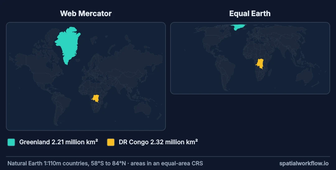
Web Mercator Greenland is 15.39× DR Congo
The map renders. Nobody warns you. And the picture is making a claim about relative size that is wrong: two countries of almost the same area, one drawn several times the size of the other.
The default is whatever CRS the data arrived in — usually EPSG:4326 for a download, EPSG:3857 if it came from a web service. Neither was chosen for your map, and both distort in specific, predictable ways that show up most in exactly the regions people look at first.
Quick answer
Choose the projection from the extent of your data and what the map claims:
gb.to_crs(27700).plot() # a national map of Great Britain, in its own grid| Your extent | Use | Why |
|---|---|---|
| a city or site | the local national grid, or UTM | metres, minimal distortion |
| one country | that country's official CRS (EPSG:27700, 2154, 25832…) | designed for it |
| a continent | an equal-area projection (EPSG:3035 for Europe) | comparable areas |
| the world, thematic | Equal Earth (EPSG:8857) or Mollweide | areas comparable |
| the world, with a basemap | Web Mercator (EPSG:3857) | tiles require it |
| never | EPSG:4326 for anything measured | degrees are not a length |
# thematic world map — areas must be comparable
world.to_crs("EPSG:8857").plot(column="pop_density", legend=True)

# national map — the country's own grid
gb.to_crs(27700).plot()

# with a basemap — Web Mercator, because the tiles are
import contextily as cx
ax = manchester.to_crs(3857).plot(alpha=0.6)
cx.add_basemap(ax, source=cx.providers.CartoDB.Positron)
What plotting degrees does, and what Web Mercator stretches
1. Understand what plotting EPSG:4326 actually does
A .plot() on unprojected data treats longitude as x and latitude as y, with no transformation at all. That is a real projection — the Plate Carrée — and it has a specific, severe distortion: east–west distances are stretched by 1/cos(latitude).
import geopandas as gpd
import numpy as np

for lat in [0, 30, 51.5, 60, 70]:
    print(f"{lat:>5}°N   1° of longitude = {111.32 * np.cos(np.radians(lat)):6.1f} km"
          f"   stretch factor {1/np.cos(np.radians(lat)):.2f}×")
0°N 1° of longitude = 111.3 km stretch factor 1.00×
30°N 1° of longitude = 96.4 km stretch factor 1.15×
51.5°N 1° of longitude = 69.3 km stretch factor 1.61×
60°N 1° of longitude = 55.7 km stretch factor 2.00×
70°N 1° of longitude = 38.1 km stretch factor 2.92×
At London's latitude, a degree of longitude is 69 km and a degree of latitude is 111 km — but the plot draws them the same width. Britain appears 61% wider than it is. At 60°N the error doubles.
The one-line remedy when you must stay in degrees:
ax = gb.plot()
ax.set_aspect(1 / np.cos(np.radians(gb.union_all().centroid.y)))
print(f"aspect set to {ax.get_aspect():.2f}")
aspect set to 1.71
This is a display fix only. It corrects the picture; it does not make gdf.area mean anything.
2. Know Web Mercator's specific distortion
Web Mercator (EPSG:3857) is conformal: it preserves local angles and shapes, which is exactly right for a navigable slippy map — a road crossing at 90° looks like 90° at every zoom. The cost is area, inflated by 1/cos²(latitude):
for lat, place in [(0, "Kenya"), (51.5, "London"), (60, "Oslo"), (71, "Tromsø")]:
    print(f"{place:<8} {lat:>5}°  appears {1/np.cos(np.radians(lat))**2:5.1f}× its true area")
Kenya 0° appears 1.0× its true area
London 51.5° appears 2.6× its true area
Oslo 60° appears 4.0× its true area
Tromsø 71° appears 9.4× its true area
This is why Greenland (2.2 M km²) looks the size of Africa (30 M km²) on a web map. For navigation it does not matter. For a choropleth it makes the map argue for a conclusion the data does not support — the visual weight of a region becomes a function of its latitude.
Use Web Mercator when you need basemap tiles, and only then. Every tile provider serves EPSG:3857, so reprojecting the data to match is not optional — see how to add a basemap with contextily.
3. Match the projection property to the map's claim
Every projection preserves some properties and destroys others. You cannot have them all — that is a theorem, not a limitation of the software.
| Property preserved | Family | Use for |
|---|---|---|
| area (equal-area) | Albers, Lambert Azimuthal, Mollweide, Equal Earth | choropleths, density, any "how much" map |
| shape locally (conformal) | Mercator, Lambert Conformal Conic, Stereographic | navigation, angles, slippy maps |
| distance from a point | Azimuthal Equidistant | travel time, range rings, "distance from here" |
| direction from a point | Azimuthal (Gnomonic) | flight paths, signal coverage |
| compromise | Robinson, Winkel Tripel, Natural Earth | reference world maps, no strong claim |
The single most useful rule: if the map's message is about quantity per area, use an equal-area projection. A choropleth of population density in Web Mercator is a picture that contradicts its own legend.
# a density map, honestly
world.to_crs("EPSG:8857").plot(column="pop_density", scheme="quantiles", k=6, legend=True)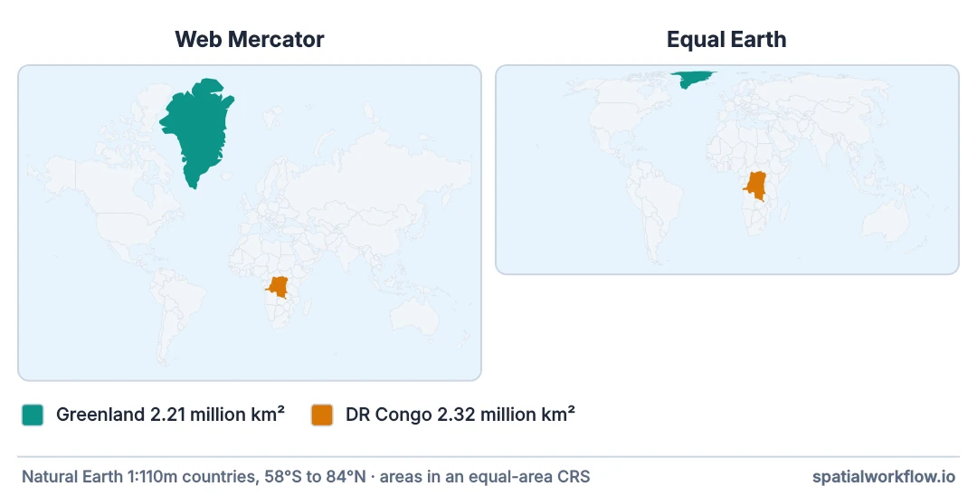
4. Choose a projected CRS for a national or regional map
Most countries have an official projected CRS, designed to keep distortion under about 1 part in 2,500 across the country:
| Area | EPSG | Notes |
|---|---|---|
| Great Britain | 27700 | OSGB36 / British National Grid |
| Ireland | 2157 | Irish Transverse Mercator |
| France | 2154 | RGF93 / Lambert-93 |
| Germany | 25832 / 25833 | ETRS89 / UTM 32N, 33N |
| Netherlands | 28992 | Amersfoort / RD New |
| Contiguous USA | 5070 | NAD83 / Conus Albers (equal-area) |
| Europe (thematic) | 3035 | ETRS89-LAEA — equal-area |
| Europe (conformal) | 3034 | ETRS89-LCC |
| Anywhere | 326xx / 327xx | UTM zone: 32600 + zone north, 32700 + zone south |
def utm_epsg(gdf):
    """EPSG code of the UTM zone containing this layer's centroid."""
    c = gdf.to_crs(4326).union_all().centroid
    zone = int((c.x + 180) // 6) + 1
    return (32600 if c.y >= 0 else 32700) + zone

print(utm_epsg(manchester))
32630
Manchester is in zone 30 north. UTM is a reasonable default for anything up to a few hundred kilometres across. Beyond one zone — six degrees of longitude — distortion at the edges grows and a conic projection fits better. Full treatment in how to choose the right projected CRS.
5. Centre the projection on your data
For a continent-scale or unusual extent, a projection centred on the area beats any standard code:
gdf = europe
gdf4326 = gdf.to_crs(4326)
c = gdf4326.union_all().centroid
minx, miny, maxx, maxy = gdf4326.total_bounds

# Lambert Azimuthal Equal Area, centred on the data
laea = f"+proj=laea +lat_0={c.y:.4f} +lon_0={c.x:.4f} +datum=WGS84 +units=m +no_defs"

# Albers Equal Area — better for a wide east-west extent
albers = (f"+proj=aea +lat_1={miny + (maxy-miny)/6:.4f} "
          f"+lat_2={maxy - (maxy-miny)/6:.4f} "
          f"+lat_0={c.y:.4f} +lon_0={c.x:.4f} +datum=WGS84 +units=m +no_defs")

ax = gdf.to_crs(albers).plot()
print(albers)
+proj=aea +lat_1=42.3001 +lat_2=73.0378 +lat_0=52.1689 +lon_0=15.4408 +datum=WGS84 +units=m +no_defs
The standard parallels at one-sixth in from each edge is the classic rule of thumb, and it keeps scale error small across the whole extent rather than minimal in the middle and poor at the edges.
The same data in four projections, with distortion measured
The data used on this page
Natural Earth's 1:110m countries for the world maps, with population density computed in Equal Earth; Eurostat's GISCO NUTS 2 regions (2024, 1:20 million) for Europe, and the mainland subset of them; and ONS boundaries for Great Britain and for the ten boroughs of Greater Manchester.
import io

import geopandas as gpd
import numpy as np
import requests

world = gpd.read_file("https://naciscdn.org/naturalearth/110m/cultural/ne_110m_admin_0_countries.zip",
                      columns=["NAME", "CONTINENT", "POP_EST"]).rename(columns=str.lower)
world["pop_density"] = world["pop_est"] / (world.to_crs(8857).area / 1e6)       # people per km²
world.to_file("world.gpkg")

nuts2 = gpd.read_file("https://gisco-services.ec.europa.eu/distribution/v2/nuts/geojson/"
                      "NUTS_RG_20M_2024_4326_LEVL_2.geojson")
nuts2.to_file("nuts2.gpkg")

europe = nuts2.cx[-25:45, 34:72].reset_index(drop=True)                        # drops the Canaries, Madeira, French overseas
europe.to_file("europe.gpkg")

ONS = "https://services1.arcgis.com/ESMARspQHYMw9BZ9/arcgis/rest/services"


def ons(layer, where, fields):
    r = requests.get(f"{ONS}/{layer}/FeatureServer/0/query", timeout=120,
                     params={"where": where, "outFields": fields, "outSR": 4326, "f": "geojson"})
    return gpd.read_file(io.BytesIO(r.content))


gb = ons("Countries_December_2024_Boundaries_UK_BUC", "CTRY24NM <> 'Northern Ireland'", "CTRY24NM")
GM = ["Bolton", "Bury", "Manchester", "Oldham", "Rochdale", "Salford", "Stockport", "Tameside", "Trafford", "Wigan"]
manchester = ons("Local_Authority_Districts_DEC_2025_Boundaries_UK_BGC",
                 "LAD25NM IN (" + ",".join(f"'{n}'" for n in GM) + ")", "LAD25NM")
manchester.to_file("manchester.gpkg")
print(f"{len(world)} countries, {len(nuts2)} NUTS 2 regions ({len(europe)} mainland), "
      f"{len(gb)} GB nations, {len(manchester)} Greater Manchester boroughs")
177 countries, 299 NUTS 2 regions (292 mainland), 3 GB nations, 10 Greater Manchester boroughs
Example 1: pick the projection automatically
import geopandas as gpd
import numpy as np

NATIONAL = {"GB": 27700, "IE": 2157, "FR": 2154, "DE": 25832, "NL": 28992, "US": 5070}

def display_crs(gdf, *, purpose="thematic", country=None):
    """Return a CRS suited to this layer's extent and the map's purpose."""
    if purpose == "basemap":
        return 3857                                    # tiles leave no choice

    g = gdf.to_crs(4326)
    minx, miny, maxx, maxy = g.total_bounds
    span_deg = max(maxx - minx, maxy - miny)
    c = g.union_all().centroid

    if country and country in NATIONAL:
        return NATIONAL[country]

    if span_deg > 120:
        return 8857 if purpose == "thematic" else 54030   # Equal Earth / Robinson
    if span_deg > 20:
        lat1, lat2 = miny + (maxy - miny) / 6, maxy - (maxy - miny) / 6
        proj = "aea" if purpose == "thematic" else "lcc"
        return (f"+proj={proj} +lat_1={lat1:.4f} +lat_2={lat2:.4f} "
                f"+lat_0={c.y:.4f} +lon_0={c.x:.4f} +datum=WGS84 +units=m +no_defs")
    zone = int((c.x + 180) // 6) + 1
    return (32600 if c.y >= 0 else 32700) + zone

for name, purpose in [("world", "thematic"), ("europe", "thematic"), ("manchester", "reference")]:
    layer = gpd.read_file(f"{name}.gpkg")
    crs = display_crs(layer, purpose=purpose)
    print(f"{name:<12} span {layer.to_crs(4326).total_bounds}  →  {str(crs)[:60]}")
world span [-180. -90. 180. 83.64513] → 8857
europe span [-31.29250328 34.61571653 44.7986691 80.7221711 ] → +proj=aea +lat_1=42.3001 +lat_2=73.0378 +lat_0=52.1689 +lon_
manchester span [-2.73041764 53.32720035 -1.90962083 53.68573403] → 32630
The purpose argument is doing the real work. The same extent gets an equal-area projection for a choropleth and a conformal one for a reference map, because the two maps make different claims and different distortions are acceptable in each.
Example 2: the same data, four projections, side by side
Seeing it is more convincing than reading about it:
import matplotlib.pyplot as plt
import geopandas as gpd

world = gpd.read_file("world.gpkg")
world = world[world.continent != "Antarctica"]

PROJECTIONS = [
    ("EPSG:4326 — Plate Carrée", 4326, "east–west stretched by 1/cos(lat)"),
    ("EPSG:3857 — Web Mercator", 3857, "area inflated by 1/cos²(lat)"),
    ("EPSG:8857 — Equal Earth", 8857, "areas comparable everywhere"),
    ("ESRI:54030 — Robinson", "ESRI:54030", "compromise; nothing exact"),
]

fig, axes = plt.subplots(2, 2, figsize=(16, 10))
for ax, (title, crs, note) in zip(axes.ravel(), PROJECTIONS):
    layer = world.to_crs(crs)
    layer.plot(ax=ax, column="pop_est", scheme="quantiles", k=5,
               cmap="YlOrRd", edgecolor="white", linewidth=0.2)
    ax.set_title(f"{title}\n{note}", fontsize=10)
    ax.set_axis_off()
plt.tight_layout()
plt.savefig("projection_comparison.png", dpi=150, bbox_inches="tight")
Compare Greenland across the four panels. Under Web Mercator it rivals Africa; under Equal Earth it is a fraction of it, which is the truth. For a population map that difference is not cosmetic — it determines which regions the reader's eye treats as important.
Web Mercator's y coordinate grows without limit towards the poles — it is infinite at ±90° — which is why web maps clip at about ±85.06°. Reproject a world layer that includes Antarctica and see what happens:
import warnings

full = gpd.read_file("world.gpkg")
with warnings.catch_warnings():
    warnings.simplefilter("ignore")
    y = full.to_crs(3857).bounds[["miny", "maxy"]]
print(f"Antarctica in EPSG:3857: miny {y['miny'].min():.3g}, finite: {np.isfinite(y['miny'].min())}")
clipped = full.clip_by_rect(-180, -85.06, 180, 85.06)                # clip before reprojecting to 3857
print(f"after clipping to ±85.06°: miny {gpd.GeoSeries(clipped, crs=4326).to_crs(3857).total_bounds[1]:,.0f} m")
Antarctica in EPSG:3857: miny -2.43e+08, finite: True
after clipping to ±85.06°: miny -20,048,966 m
PROJ does not raise on the pole. It returns a finite y for Antarctica of about −243,000 km — six times the Earth's circumference — and a plot of it is a thin sliver of world above a vast smear of ice. Clipped at the web-map limit, the whole map fits within ±20,049 km, the square every web map is built on.
Example 3: measuring the distortion at your own extent
Rather than trusting a rule of thumb, measure what your chosen projection does to your data:
import geopandas as gpd
import numpy as np
from shapely.geometry import Point

def distortion_report(gdf, crs, samples=200):
    """Compare projected area against geodesic area for sample features."""
    from pyproj import Geod
    geod = Geod(ellps="WGS84")

    g4326 = gdf.to_crs(4326)
    sample = g4326.sample(min(samples, len(g4326)), random_state=0)
    projected = sample.to_crs(crs)

    true_area = np.array([abs(geod.geometry_area_perimeter(g)[0]) for g in sample.geometry])
    proj_area = projected.geometry.area.to_numpy()
    ratio = proj_area / np.where(true_area == 0, np.nan, true_area)

    print(f"CRS {str(crs)[:48]}")
    print(f"  area ratio  min {np.nanmin(ratio):.3f}  median {np.nanmedian(ratio):.3f}  "
          f"max {np.nanmax(ratio):.3f}")
    print(f"  worst error {100 * np.nanmax(np.abs(ratio - 1)):.1f}%")
    return ratio

europe = gpd.read_file("nuts2.gpkg")
for crs in [3857, 3035, 4326]:
    distortion_report(europe, crs)
CRS 3857
area ratio min 1.091 median 2.177 max 26.860
worst error 2586.0%
CRS 3035
area ratio min 1.000 median 1.000 max 1.000
worst error 0.0%
CRS 4326
area ratio min 0.000 median 0.000 max 0.000
worst error 100.0%
Three readings. Web Mercator inflates European regions by between about 1.1× and 27× — the extreme is Svalbard, at nearly 80°N — so a choropleth in it is comparing regions on inconsistent visual footing. EPSG:3035, Europe's official equal-area CRS, matches the ellipsoidal area to within rounding, which is as good as it gets. And EPSG:4326 produces areas in square degrees, a number with no relationship to square metres at all, which is why the ratio is effectively zero.
pyproj.Geod.geometry_area_perimeter computes area on the ellipsoid, which is the ground truth to compare against.
No projection preserves everything
A projection is a function from the curved surface of the earth to a flat plane, and no such function can preserve everything. This is a mathematical result, not a software limitation: a sphere has intrinsic curvature and a plane does not, so any mapping between them must stretch, compress or tear. Every projection is a choice about what to sacrifice.
The three properties that matter for maps are area, shape and distance, and preserving any one costs the others.
Equal-area projections keep the ratio of areas exact everywhere. They pay in shape: Mollweide's outer regions are visibly squashed, Albers' are sheared. For a choropleth this is the right trade, because the reader's judgement of "how much" comes from visual area. A region drawn twice its true size carries twice the weight regardless of its colour.
Conformal projections keep local angles exact, so small shapes look right and a rectangle of streets stays rectangular. They pay in area, and Mercator pays extravagantly: 1/cos²(latitude), which is 4× at 60°N and unbounded at the poles. This is the correct trade for navigation — Mercator's defining property is that a line of constant compass bearing is a straight line — and the wrong trade for anything thematic.
Web Mercator's dominance is a historical accident with real consequences. It won because it is cheap to compute at tile boundaries and because Google chose it in 2005. It is now the only projection every tile provider serves, so any map with a basemap must use it, and any thematic map with a basemap inherits its area distortion. When the theme is quantitative and the geography spans latitudes, that is a genuine conflict, and the honest resolutions are to drop the basemap, or to normalise the quantity so area is not what the reader is judging.
And EPSG:4326 is not a projection at all. It is a geographic coordinate system: angles on an ellipsoid. Plotting it treats degrees as if they were a planar coordinate, which silently applies the Plate Carrée projection — a defensible projection near the equator and a poor one at 55°N, where it stretches east–west by 61%. The more serious problem is that gdf.area and gdf.distance then return square degrees and degrees, numbers with no fixed relationship to metres. GeoPandas warns about this once, and it is worth heeding — see the geographic CRS warning.
The practical consequence is a two-part rule that covers nearly every case: project for the extent, and pick the property the map's message depends on. A national map in the national grid, a thematic world map in Equal Earth, a slippy map in Web Mercator because there is no alternative. Everything else is a special case worth thinking about explicitly.
±85°, Equal Earth, ESRI codes and the antimeridian
gdf.plot()never reprojects. It draws whatever coordinates are in the frame. The CRS must be set before plotting.- Web Mercator is undefined beyond about ±85.06°. Clip with
gdf.cx[:, -85:85]before reprojecting, or you get infinities. - Equal Earth (EPSG:8857) requires PROJ 6.3+ and is the modern successor to Robinson for thematic world maps.
- ESRI codes such as
ESRI:54030(Robinson) need the string form, not an integer:to_crs("ESRI:54030"). - A projection centred on your data beats a standard code for unusual extents —
+proj=laea +lat_0=… +lon_0=…. - Data crossing the antimeridian tears in most projections. Shift longitudes or use a CRS with a different central meridian.
set_aspectfixes the picture, not the numbers. Areas and distances stay in degrees.- Matplotlib's aspect defaults to
"equal"for GeoPandas plots, which is right for projected data and wrong for 4326. - Cartopy adds graticules, coastlines and proper projection handling if you need more than GeoPandas offers.
- Print output has its own conventions — national atlases usually mandate a specific CRS. Check before choosing.
Internal links
- Coordinate reference systems explained for Python GIS — the underlying concepts
- Projected vs geographic CRS — what changes when you reproject
- How to choose the right projected CRS for your study area — the analysis-side decision
- How to add a basemap to a GeoPandas map with contextily — why basemaps force Web Mercator
- Choropleth classification explained — the other half of an honest choropleth
- How to plot maps in Python with GeoPandas and Matplotlib — the plotting basics
- GeoPandas "geometry is in a geographic CRS" warning — the warning this explains
- How to calculate area and distance in GeoPandas correctly — measuring, not drawing
FAQ
What is wrong with plotting EPSG:4326?
It applies the Plate Carrée projection silently, stretching east–west by 1/cos(latitude) — 61% at London's latitude. It also makes area and distance return degrees, which are not lengths.
Should I use Web Mercator?
Only when you need basemap tiles, which all use it. Its area inflation reaches 4× at 60°N, so it is a poor choice for any map whose message is about quantity per area.
Which projection should a choropleth use?
An equal-area one — EPSG:3035 for Europe, 5070 for the contiguous USA, 8857 for the world. Readers judge quantity by visual area, so unequal areas make the map contradict its legend.
How do I choose a CRS for one country?
Use its official projected CRS: 27700 for Great Britain, 2154 for France, 25832 for Germany. They are designed to keep distortion under about 1 part in 2,500 nationally.
Can one projection preserve area and shape together?
No. That is a mathematical impossibility for a curved surface mapped to a plane, not a limitation of any library. Compromise projections such as Robinson distribute the error instead of eliminating it.
Why does my world map break at the poles?
Web Mercator's y coordinate is infinite at ±90°. PROJ does not fail on Antarctica — it returns a finite but absurd y of about −243,000 km — so clip to about ±85° before reprojecting.
How do I check how much a projection distorts my data?
Compare projected areas against geodesic areas from pyproj.Geod.geometry_area_perimeter, as in Example 3. It takes a few lines and gives a number rather than an impression.