How to Map Population Density per km² from a Population Grid in Python

Problem statement

A population grid stores people per cell. A density map needs people per square kilometre, which means dividing by each cell's area. On an equal-area grid that is one number for every cell. On a grid in latitude and longitude, such as GHS-POP at 30 arc-seconds or WorldPop at 3 arc-seconds, cells shrink towards the poles, so the area has to be computed for each row. Then the densities need classes that work across four orders of magnitude, and a decision about whether to show where land is dense or where people live densely.

This page computes the area of every 30 arc-second row with pyproj.Geod, converts GHS-POP 2020 for the Netherlands to people per km², classes it on a logarithmic scale, measures how many people live at each density, and maps municipal densities for comparison.

Quick answer

Compute the geodesic area of one cell per row, broadcast it across the row, and divide:

geod = Geod(ellps="WGS84")
res = tf.a
lats = tf.f + tf.e * np.arange(pop.shape[0])                       # top edge of each row
row_km2 = np.array([abs(geod.polygon_area_perimeter([0, res, res, 0], [la, la, la + tf.e, la + tf.e])[0]) / 1e6 for la in lats])
cell_km2 = np.broadcast_to(row_km2[:, None], pop.shape)
density = pop / cell_km2
print(f"cell area: {row_km2.min():.3f} km2 in the north to {row_km2.max():.3f} km2 in the south")
print(f"densest cell: {density.max():,.0f} people per km2; national: {pop.sum() / cell_km2[~pop.mask].sum():,.0f}")

cell area: 0.512 km2 in the north to 0.545 km2 in the south
densest cell: 21,534 people per km2; national: 496

Within the Netherlands a cell covers 0.512 km² in the north and 0.545 km² in the south. The densest cell holds 21,534 people per km², and the country as a whole 496 per km² of land.

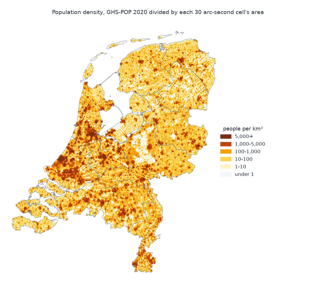
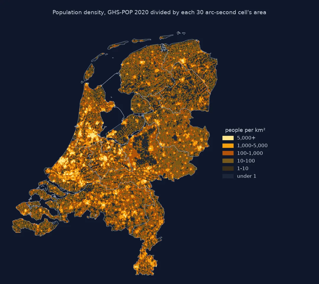
Varying cell areas, log classes, the density people live at

1. How much the cell area varies

The cell is 30 arc-seconds on each side everywhere, but a degree of longitude spans fewer kilometres the further from the equator. Compute the area at a few latitudes:

for la in (0, 30, 45, 52, 60, 70):
    a = abs(geod.polygon_area_perimeter([0, res, res, 0], [la, la, la + res, la + res])[0]) / 1e6
    print(f"latitude {la:>2}: one 30 arc-second cell = {a:.3f} km2")

latitude  0: one 30 arc-second cell = 0.855 km2
latitude 30: one 30 arc-second cell = 0.743 km2
latitude 45: one 30 arc-second cell = 0.608 km2
latitude 52: one 30 arc-second cell = 0.531 km2
latitude 60: one 30 arc-second cell = 0.432 km2
latitude 70: one 30 arc-second cell = 0.296 km2

The same cell covers 0.855 km² at the equator, 0.531 km² at 52°N and 0.296 km² at 70°N: at Dutch latitudes, dividing by the equatorial area would understate every density by 38%, and dividing by 1 km² by 47%.

2. Classes on a log scale

Densities run from under one person to tens of thousands per km². Fixed classes on powers of ten keep both ends readable, and the same classes can be used on any map:

bins = [1, 10, 100, 1_000, 5_000, 1e9]
labels = ["1-10", "10-100", "100-1,000", "1,000-5,000", "5,000+"]
d, p, a = density.compressed(), pop.compressed(), cell_km2[~pop.mask]
k = np.digitize(d, bins) - 1
T = pd.DataFrame({"class": labels, "land_km2": [a[k == i].sum() for i in range(5)], "people": [p[k == i].sum() for i in range(5)]})
T["share_of_land"], T["share_of_people"] = T.land_km2 / a.sum(), T.people / p.sum()
print(T.to_string(index=False, formatters={"land_km2": "{:,.0f}".format, "people": "{:,.0f}".format,
                                           "share_of_land": "{:.1%}".format, "share_of_people": "{:.1%}".format}))
print(f"under 1 per km2: {(d < 1).sum():,} cells, {a[d < 1].sum():,.1f} km2, {p[d < 1].sum():,.0f} people")

      class land_km2    people share_of_land share_of_people
       1-10    3,212    15,752          9.2%            0.1%
     10-100   13,501   643,969         38.5%            3.7%
  100-1,000   10,135 3,063,965         28.9%           17.6%
1,000-5,000    3,815 9,334,521         10.9%           53.7%
     5,000+      612 4,330,545          1.7%           24.9%
under 1 per km2: 7,255 cells, 3,815.2 km2, 410 people

Cells of 1,000 to 5,000 per km² cover 10.9% of the land and hold 53.7% of the people; the 1.7% of land above 5,000 per km² holds a quarter. At the other end, 38.5% of the land holds 3.7% of the people at 10 to 100 per km², and 7,255 cells, 3,815 km², hold fewer than one person per km²: 410 people in all.

3. The density people live at

The average density of the land and the density the average person lives at are different numbers. The second weights each cell by its people:

land = pop.sum() / a.sum()
lived = (d * p).sum() / p.sum()
print(f"people per km2 of land: {land:,.0f}; density at which the average person lives: {lived:,.0f}")
print(f"median person lives at {np.interp(0.5, np.cumsum(p[np.argsort(d)]) / p.sum(), np.sort(d)):,.0f} per km2")

people per km2 of land: 496; density at which the average person lives: 3,622
median person lives at 3,054 per km2

The land of the Netherlands averages 496 people per km², but the average person lives in a cell of 3,622 per km², and the median person at 3,054. Which one a map or a sentence means should be explicit; population-weighted density works this out for cities.

Density by municipality

The data used on this page

GHS-POP R2023A epoch 2020 at 30 arc-seconds (tile R4_C19), and the 2020 country and municipality boundaries from the PDOK CBS gebiedsindelingen web feature service with each municipality's population on 1 January 2020 from StatLine table 03759ned.

import io
import json
import zipfile
from pathlib import Path

import geopandas as gpd
import numpy as np
import pandas as pd
import rasterio
import requests
from pyproj import Geod
from rasterio.mask import mask

Path("data").mkdir(exist_ok=True)
name = "GHS_POP_E2020_GLOBE_R2023A_4326_30ss"
GHS = Path("data", f"{name}_V1_0_R4_C19.tif")
if not GHS.exists():
    url = f"https://jeodpp.jrc.ec.europa.eu/ftp/jrc-opendata/GHSL/GHS_POP_GLOBE_R2023A/{name}/V1-0/tiles/{GHS.stem}.zip"
    zipfile.ZipFile(io.BytesIO(requests.get(url, timeout=600).content)).extract(GHS.name, "data")
for layer in ("landsdeel", "gemeente"):
    path = Path("data", f"{layer}_2020.geojson")
    if not path.exists():
        path.write_bytes(requests.get("https://service.pdok.nl/cbs/gebiedsindelingen/2020/wfs/v1_0", timeout=300, params={
            "service": "WFS", "version": "2.0.0", "request": "GetFeature", "typeName": f"gebiedsindelingen:{layer}_gegeneraliseerd",
            "outputFormat": "application/json", "srsName": "EPSG:28992"}).content)
C = Path("data/cbs_pop_2020.json")
if not C.exists():
    C.write_bytes(requests.get("https://opendata.cbs.nl/ODataApi/odata/03759ned/TypedDataSet", timeout=300, params={
        "$filter": "Geslacht eq 'T001038' and Leeftijd eq '10000' and BurgerlijkeStaat eq 'T001019' and Perioden eq '2020JJ00' "
                   "and (substring(RegioS,0,2) eq 'GM' or substring(RegioS,0,2) eq 'NL')",
        "$select": "RegioS,BevolkingOp1Januari_1"}).content)
OFF = {r["RegioS"].strip(): r["BevolkingOp1Januari_1"] for r in json.loads(C.read_text())["value"] if r["BevolkingOp1Januari_1"]}
NL = gpd.read_file("data/landsdeel_2020.geojson").dissolve()
GM = gpd.read_file("data/gemeente_2020.geojson")
with rasterio.open(GHS) as src:
    a, tf = mask(src, NL.to_crs(src.crs).geometry, crop=True, filled=False)
pop = a[0]
print(f"{pop.count():,} cells inside the Netherlands, {pop.sum():,.0f} people; rows from {tf.f:.3f} N down to {tf.f + tf.e * pop.shape[0]:.3f} N")

66,493 cells inside the Netherlands, 17,389,161 people; rows from 53.558 N down to 50.750 N

The clipped grid has 66,493 cells and 17,389,161 people, in rows from 53.558°N to 50.750°N.

Example 1: density by municipality

The same measure for areas is official population over land area. Compute it in the Dutch RD New grid, which is close to equal-area at this scale:

GM["people"] = GM.statcode.map(OFF)
GM["km2"] = GM.area / 1e6
GM["density"] = GM.people / GM.km2
fmt = {"people": "{:,}".format, "km2": "{:,.1f}".format, "density": "{:,.0f}".format}
print(GM.nlargest(3, "density")[["statnaam", "people", "km2", "density"]].to_string(index=False, formatters=fmt))
print(GM.nsmallest(3, "density")[["statnaam", "people", "km2", "density"]].to_string(index=False, header=False, formatters=fmt))
print(f"country: {GM.people.sum() / GM.km2.sum():,.0f} per km2 of land")

     statnaam  people  km2 density
's-Gravenhage 545,838 85.6   6,378
       Leiden 125,099 23.3   5,366
      Haarlem 162,902 32.0   5,085
Schiermonnikoog   947 39.8 24
       Vlieland 1,155 40.4 29
   Terschelling 4,888 85.5 57
country: 496 per km2 of land

Den Haag is the densest municipality at 6,378 people per km² of land, followed by Leiden and Haarlem; the Wadden islands Schiermonnikoog, Vlieland and Terschelling are the least dense, from 24 to 57. Official population over municipal land gives the same 496 per km² for the country as the grid.

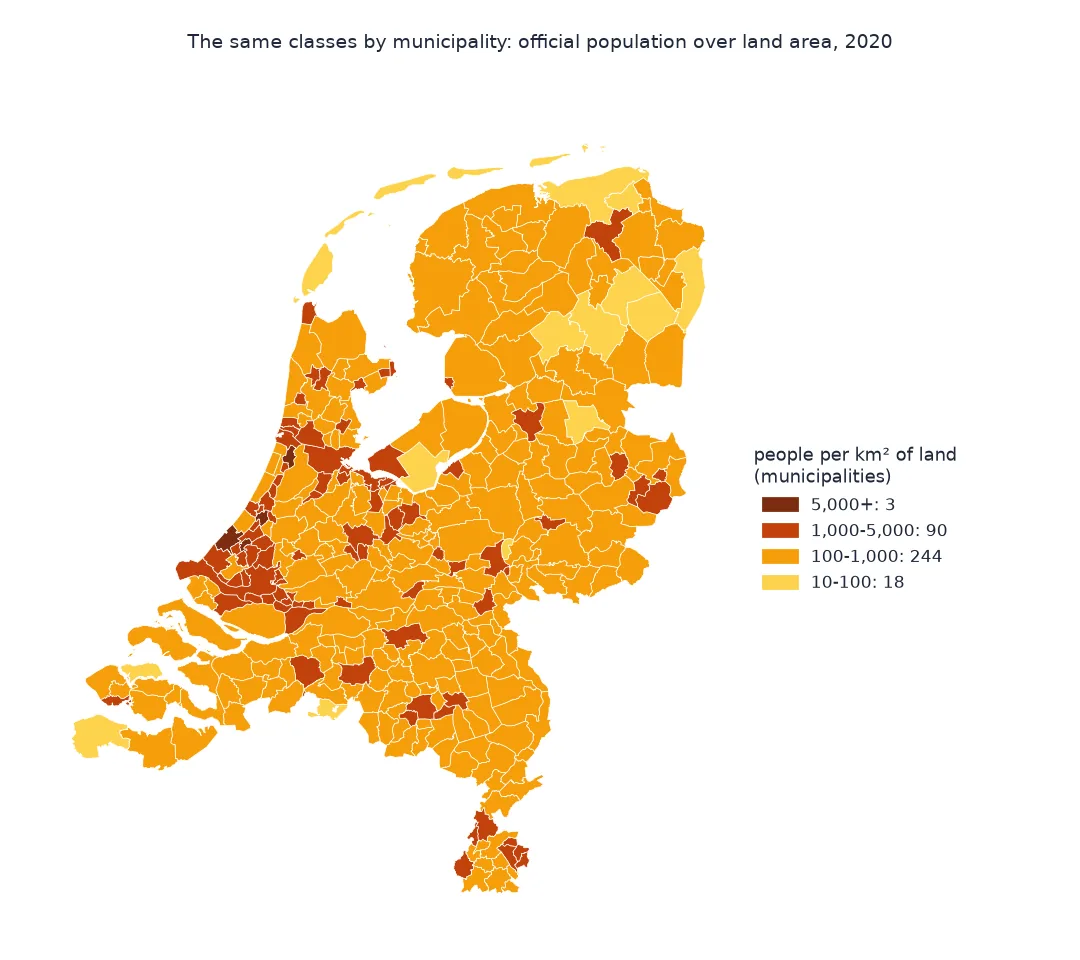
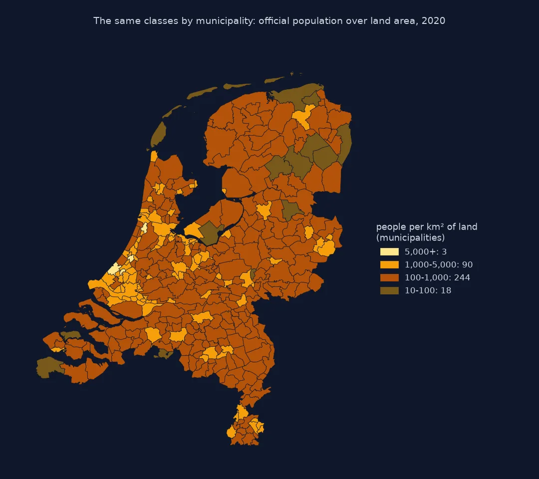
Density is a ratio, and both halves need care

Density is a ratio, and both halves need care. The numerator, people per cell, is what the grid provides. The denominator, the area of the cell, is a property of the grid's geometry: constant on an equal-area grid such as GHS-POP's Mollweide layers or a national grid, variable by row on a latitude-longitude grid. At 52°N a 30 arc-second cell covers 0.53 km², not 1 km² and not the 0.86 km² it covers at the equator, and treating it as either misstates every density in the country by the same factor.

The resolution of the grid sets what "density" means. At 1 km, a city block and the park beside it are averaged into one cell; at 100 m they are separate. The densest 30 arc-second cell in the Netherlands holds 21,534 people per km², while the census grid page finds a 100 m square at 218,000. Neither is wrong: they are densities of different areas. Compare densities only at one resolution, and say which one.

Land area, equal-area grids and log floors

• Land or total area: a coastal cell that is half sea has a land density twice its cell density; mask water or divide by land area where it matters.
• Equal-area alternatives: GHS-POP is also published in Mollweide at 100 m and 1 km, where every cell is 0.01 or 1 km²; using that layer avoids the area calculation entirely.
• Log classes need a floor: cells with zero people have no logarithm; give them their own class rather than dropping them.
• Cell area formula: on a sphere a cell covers R² Δλ (sin φ₂ − sin φ₁); the ellipsoidal Geod calculation used here differs from it by a fraction of a percent.

Internal links

• Fixing population densities that are wrong on latitude-longitude grids — what goes wrong without the area
• How to compute population-weighted density in Python — the density people live at, by city
• Why density depends on the boundary — the same effect for polygons

FAQ

How do I convert a population raster to density in Python?

Divide each cell by its area in km². On a projected equal-area grid that is one constant; on a latitude-longitude grid compute the area per row, for example with pyproj.Geod.polygon_area_perimeter, and broadcast it.

How big is a 30 arc-second cell?

About 0.86 km² at the equator, 0.53 km² at 52°N in the Netherlands, and 0.29 km² at 70°N.

What classes should a population density map use?

Logarithmic ones, such as powers of ten with an extra break at 5,000 per km², because densities span four or five orders of magnitude.

What is the population density of the Netherlands?

About 500 people per km² of land, from official population and municipal land area in 2020; the average person lives at a much higher density.