
Choosing a Python Map Library: Folium, Plotly, pydeck, Lonboard and Cartopy Explained
On this page
Problem statement
Python has more ways to make a map than any other language: GeoPandas with matplotlib, Cartopy, Folium, Plotly, pydeck and lonboard are all mature, and each tutorial uses a different one. They are not interchangeable. Some produce images, some web pages. Some draw with the browser's DOM, others on the GPU. Some carry the data inside the file, others load it later. The right choice depends on who will see the map, in what medium, and how many features it has to show.
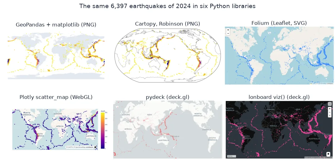
This page makes the same map, every magnitude 4.5 and larger earthquake of 2024, with six libraries. It compares what each produces, how the output grows as the data does, and what each page needs from the network when it opens, and ends with a decision table.
Quick answer
Build the same map six ways and compare the outputs:
fig, ax = plt.subplots(figsize=(10, 5)); W.plot(ax=ax, color="#e2e8f0", lw=0)
ax.scatter(Q.longitude, Q.latitude, s=3, c=Q.depth, cmap="plasma_r", vmin=0, vmax=300); ax.set_axis_off()
fig.savefig("data/m_matplotlib.png", dpi=100, bbox_inches="tight"); plt.close(fig)

fig = plt.figure(figsize=(10, 5)); ax = plt.axes(projection=ccrs.Robinson(central_longitude=180)); ax.set_global(); ax.coastlines(linewidth=0.4)
ax.scatter(Q.longitude, Q.latitude, s=3, c=Q.depth, cmap="plasma_r", vmin=0, vmax=300, transform=ccrs.PlateCarree())
fig.savefig("data/m_cartopy.png", dpi=100, bbox_inches="tight"); plt.close(fig)

m = folium.Map(location=[20, 10], zoom_start=2)
folium.GeoJson(G[["mag", "depth", "geometry"]], marker=folium.CircleMarker(radius=2, weight=0, fill=True, fill_opacity=0.7)).add_to(m)
m.save("data/m_folium.html")

px.scatter_map(Q, lat="latitude", lon="longitude", color="depth", range_color=(0, 300), zoom=0.6).write_html("data/m_plotly.html", include_plotlyjs="cdn")

pdk.Deck(layers=[pdk.Layer("ScatterplotLayer", Q[["longitude", "latitude", "depth"]], get_position=["longitude", "latitude"], get_radius=30000,
                           get_fill_color=[239, 68, 68, 160])], initial_view_state=pdk.ViewState(latitude=10, longitude=150, zoom=0.8),
         map_style="light").to_html("data/m_pydeck.html", open_browser=False, notebook_display=False)

viz(G[["mag", "depth", "geometry"]]).to_html("data/m_lonboard.html")

for f in ("m_matplotlib.png", "m_cartopy.png", "m_folium.html", "m_plotly.html", "m_pydeck.html", "m_lonboard.html"):
    print(f"{f:>16}: {Path('data/' + f).stat().st_size / 1e6:6.2f} MB")
m_matplotlib.png: 0.10 MB
m_cartopy.png: 0.14 MB
m_folium.html: 1.25 MB
m_plotly.html: 0.22 MB
m_pydeck.html: 0.71 MB
m_lonboard.html: 4.77 MB
The two static images are 0.10 and 0.14 MB. Among the web pages, Plotly's is the smallest at 0.22 MB, followed by pydeck at 0.71 MB and Folium at 1.25 MB. Lonboard's is the largest, 4.77 MB, because the page carries its own JavaScript widget.
Output size, network requests, the decision
1. How the output grows with the data
Repeat the four web libraries with 100,000 named places from the USGS Geographic Names Information System, and compare the bytes each needs per point:
S = P.sample(100_000, random_state=0)
mm = folium.Map(location=[39, -98], zoom_start=4)
folium.GeoJson(S[["geometry"]], marker=folium.CircleMarker(radius=1, weight=0, fill=True)).add_to(mm); mm.save("data/s_folium.html")
px.scatter_map(lat=S.geometry.y, lon=S.geometry.x).write_html("data/s_plotly.html", include_plotlyjs="cdn")
pdk.Deck(layers=[pdk.Layer("ScatterplotLayer", pd.DataFrame({"lon": S.geometry.x, "lat": S.geometry.y}), get_position=["lon", "lat"], get_radius=2000)],
         map_style="light").to_html("data/s_pydeck.html", open_browser=False, notebook_display=False)
viz(S[["geometry"]]).to_html("data/s_lonboard.html")
for lib in ("folium", "plotly", "pydeck", "lonboard"):
    small, big = Path(f"data/m_{lib}.html").stat().st_size, Path(f"data/s_{lib}.html").stat().st_size
    print(f"{lib:>8}: {big / 1e6:6.2f} MB for 100,000 points; {(big - small) / (100_000 - len(Q)):5.1f} bytes per extra point")
folium: 18.80 MB for 100,000 points; 187.5 bytes per extra point
plotly: 2.26 MB for 100,000 points; 21.8 bytes per extra point
pydeck: 7.90 MB for 100,000 points; 76.9 bytes per extra point
lonboard: 7.54 MB for 100,000 points; 29.6 bytes per extra point
Per extra point, Plotly adds 21.8 bytes, lonboard 29.6, pydeck 76.9 and Folium 187.5, so at 100,000 points the pages range from 2.26 MB for Plotly to 18.80 MB for Folium. Lonboard's fixed overhead is large, but its cost per point is low. Folium's GeoJSON with a style for every feature is the most expensive.
2. What each page asks the network for
A saved web map is not self-contained unless it says so. List the external hosts each HTML file loads scripts, styles or tiles from:
import re
for lib in ("folium", "plotly", "pydeck", "lonboard"):
    html = Path(f"data/m_{lib}.html").read_text(errors="ignore")
    hosts = sorted(set(re.findall(r'(?:src|href)="https?://([^/"]+)', html)))
    print(f"{lib:>8}: {', '.join(hosts) if hosts else '(none in src/href attributes)'}")
folium: cdn.jsdelivr.net, cdnjs.cloudflare.com, code.jquery.com, netdna.bootstrapcdn.com
plotly: cdn.plot.ly
pydeck: api.tiles.mapbox.com, maxcdn.bootstrapcdn.com, unpkg.com
lonboard: cdn.jsdelivr.net, cdnjs.cloudflare.com
Every web page loads code from content delivery networks when it opens: four hosts for Folium, Plotly's own CDN, unpkg and Bootstrap for pydeck (plus a Mapbox stylesheet), and jsDelivr and cdnjs for lonboard. Basemap tiles come on top of these. None of them works offline as saved.
3. The decision
| You need | Use |
|---|---|
| a figure for a paper, report or slide | GeoPandas + matplotlib, or Cartopy for projections and globes |
| a quick interactive look at a GeoDataFrame | gdf.explore() (Folium) |
| a shareable web map with popups and a few thousand features | Folium |
| charts and maps in one dashboard, animation, hover templates | Plotly |
| 3D columns, hexagons, arcs | pydeck |
| hundreds of thousands to millions of features in a notebook | lonboard |
What each library's output is
The data used on this page
Every earthquake of magnitude 4.5 or more worldwide in 2024 from the USGS FDSN event service, the Natural Earth 1:110m countries for the static base, and the national file of the GNIS Domestic Names for the scaling test.
import zipfile
from pathlib import Path

import cartopy.crs as ccrs
import folium
import geopandas as gpd
import matplotlib
matplotlib.use("Agg")
import matplotlib.pyplot as plt
import pandas as pd
import plotly.express as px
import pydeck as pdk
import requests
from lonboard import viz

Path("data").mkdir(exist_ok=True)
def cached(path, url, timeout=900):
    p = Path(path)
    if not p.exists():
        r = requests.get(url, timeout=timeout, headers={"User-Agent": "spatialworkflow-guide/1.0"})
        r.raise_for_status()
        p.write_bytes(r.content)
    return p
q = Path("data/quakes_m45_2024.csv")
if not q.exists():
    r = requests.get("https://earthquake.usgs.gov/fdsnws/event/1/query", timeout=600,
                     params=dict(format="csv", starttime="2024-01-01", endtime="2025-01-01", minmagnitude=4.5, orderby="time-asc"))
    r.raise_for_status()
    q.write_bytes(r.content)
Q = pd.read_csv(q)
Q = Q[Q["type"] == "earthquake"].reset_index(drop=True)
G = gpd.GeoDataFrame(Q, geometry=gpd.points_from_xy(Q.longitude, Q.latitude), crs=4326)
W = gpd.read_file(cached("data/ne_110m_admin_0_countries.zip", "https://naciscdn.org/naturalearth/110m/cultural/ne_110m_admin_0_countries.zip"))
with zipfile.ZipFile(cached("data/DomesticNames_National_Text.zip", "https://prd-tnm.s3.amazonaws.com/StagedProducts/GeographicNames/DomesticNames/DomesticNames_National_Text.zip")) as z:
    N = pd.read_csv(z.open("Text/DomesticNames_National.txt"), sep="|", low_memory=False)
N = N[N.prim_lat_dec.between(-90, 90) & N.prim_long_dec.between(-180, 180) & ~((N.prim_lat_dec == 0) & (N.prim_long_dec == 0))]
P = gpd.GeoDataFrame(geometry=gpd.points_from_xy(N.prim_long_dec, N.prim_lat_dec), crs=4326)
print(f"{len(Q):,} earthquakes; {len(P):,} GNIS names with coordinates")
6,397 earthquakes; 969,148 GNIS names with coordinates
The test data is 6,397 earthquakes, plus 969,148 GNIS names with usable coordinates for the scaling test.
Example 1: what each output is
Static images are pixels; web maps are programs. Check the format and what a reader can do with each:
from PIL import Image
for f in ("m_matplotlib.png", "m_cartopy.png"):
    im = Image.open(f"data/{f}")
    print(f"{f:>16}: {im.format} image {im.size[0]} x {im.size[1]} px; opens anywhere, prints, no zoom or hover")
for lib, draws in (("folium", "Leaflet, SVG in the DOM"), ("plotly", "Plotly.js with MapLibre, WebGL"), ("pydeck", "deck.gl, WebGL"), ("lonboard", "deck.gl, WebGL, binary data")):
    print(f"{'m_' + lib + '.html':>16}: HTML page; draws with {draws}")
m_matplotlib.png: PNG image 795 x 400 px; opens anywhere, prints, no zoom or hover
m_cartopy.png: PNG image 779 x 405 px; opens anywhere, prints, no zoom or hover
m_folium.html: HTML page; draws with Leaflet, SVG in the DOM
m_plotly.html: HTML page; draws with Plotly.js with MapLibre, WebGL
m_pydeck.html: HTML page; draws with deck.gl, WebGL
m_lonboard.html: HTML page; draws with deck.gl, WebGL, binary data
The static outputs are PNG images of about 800 × 400 pixels. The four web pages are programs that draw with Leaflet's SVG, or with WebGL through MapLibre or deck.gl.
Image renderers against web renderers
The libraries fall into two families. GeoPandas' plot, matplotlib and Cartopy render an image in Python: what you save is what everyone sees, with any projection, at any resolution, ready for print, but with no zoom and no hover. Folium, Plotly, pydeck and lonboard write a web page that a browser turns into a map each time it opens. The reader can zoom, pan and query, and the page depends on the browser, the network for tiles and scripts, and the hardware for drawing. Within the web family the split is in how the data travels and how it is drawn. Folium writes GeoJSON text and draws with Leaflet in the DOM. Plotly and pydeck write JSON and draw with WebGL. Lonboard sends compact binary columns straight to the GPU.
Those mechanics decide where each library stops being comfortable. Text formats cost from about 20 to almost 190 bytes per point, and DOM drawing costs an element per feature, so Folium suits thousands of features rather than hundreds of thousands. WebGL libraries draw far more, and lonboard's binary transfer makes a million points practical. Beyond capability, the choice is about the audience: a printed report needs a static map, a dashboard needs Plotly's integration with charts, and a notebook exploration of a large dataset needs lonboard. Most projects end up using two: one static, one interactive.
Basemaps, offline pages and apps
- Basemaps: every web library depends on a tile provider; CARTO's raster tiles now need a key, see the API KEY REQUIRED fix.
- Offline pages: Plotly can embed its JavaScript (
include_plotlyjs=True); Folium, pydeck and lonboard pages load libraries or tiles from the network. - Static images from web libraries: Plotly exports PNG and SVG through Kaleido; Folium needs a headless browser, see saving a Folium map as an image.
- Apps: for a map inside an application, see choosing a framework for a map app.
Internal links
- How to make an interactive map with GeoPandas explore() — the quickest start
- Interactive vs static maps explained — the first decision
- SVG, canvas and WebGL explained — why the web libraries scale differently
FAQ
What is the best Python library for maps?
There is no single best: matplotlib or Cartopy for static figures, Folium for simple web maps, Plotly for dashboards, pydeck for 3D, and lonboard for very large data.
Folium or Plotly?
Folium for Leaflet maps with popups, layer controls and plugins; Plotly when the map sits beside charts, needs animation, or should share a dashboard's styling.
Which Python map library handles the most points?
Lonboard, which sends binary data to the GPU; pydeck and Plotly handle tens to hundreds of thousands, Folium thousands.
Which library should I use for a map in a paper?
GeoPandas with matplotlib, or Cartopy when the projection matters; both save vector or high-resolution images.