How to Make a Map With Cartopy in Python

Problem statement

Cartopy is the standard library for publication-quality static maps in Python. It adds map projections, coastlines and gridlines to matplotlib, and it can centre a world map on the Pacific, draw a regional map in a conformal projection or show the globe from space. It also has one rule that causes most of the questions about it: the projection of the axes and the coordinate system of the data are separate, and plotting longitude and latitude without saying so puts everything in the wrong place.

This page maps every magnitude 4.5 and larger earthquake of 2024 with Cartopy: a Pacific-centred world map in the Robinson projection, a regional map of Japan in a Lambert conformal projection, Natural Earth borders and labelled gridlines, and a check of what happens without transform.

Quick answer

Create axes with a projection, add features, and plot the data with transform=ccrs.PlateCarree() because the data is longitude and latitude:

import cartopy.crs as ccrs
import cartopy.feature as cfeature
fig = plt.figure(figsize=(10, 5.4))
ax = plt.axes(projection=ccrs.Robinson(central_longitude=180))
ax.set_global()
ax.add_feature(cfeature.LAND, facecolor="#e2e8f0"); ax.add_feature(cfeature.OCEAN, facecolor="#e8f4fd"); ax.coastlines(linewidth=0.4)
sc = ax.scatter(Q.longitude, Q.latitude, s=(Q.mag - 4) ** 2 * 3, c=Q.depth, cmap="plasma_r", vmin=0, vmax=300,
                transform=ccrs.PlateCarree(), linewidths=0, alpha=0.7)
fig.colorbar(sc, ax=ax, shrink=0.6, label="depth (km)")
fig.savefig("data/cartopy_world.png", dpi=150, bbox_inches="tight"); plt.close(fig)
print(f"projection: {ax.projection.to_proj4()}")
print(f"PNG {Image.open('data/cartopy_world.png').size}")

projection: +proj=robin +lon_0=180 +x_0=0 +y_0=0 +R=6378137 +units=m +no_defs +type=crs
PNG (1119, 501)

The axes use the Robinson projection centred on 180°, in metres on a sphere of radius 6,378,137 m. The saved PNG is 1119 × 501 pixels.

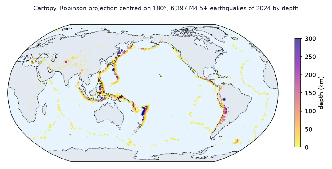
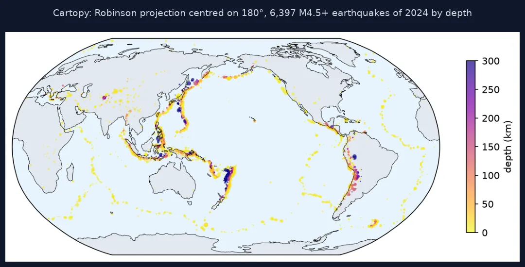
Projection and transform, a regional map, projections compared

1. projection and transform

projection= sets how the map is drawn; transform= says what the data's coordinates are. Without transform, Cartopy reads the numbers as metres in the map projection:

lon, lat = 145.4596, 17.6625                                                # the first earthquake of 2024
x, y = ax.projection.transform_point(lon, lat, ccrs.PlateCarree())
print(f"with transform:    ({x / 1000:,.0f} km, {y / 1000:,.0f} km) in Robinson coordinates")
print(f"without transform: ({lon:.0f} m, {lat:.0f} m) from the map centre at 180°, 0°")
far = np.hypot(Q.longitude, Q.latitude).max()
print(f"without transform every earthquake lands within {far:.0f} m of the centre")

with transform:    (-3,218 km, 1,889 km) in Robinson coordinates
without transform: (145 m, 18 m) from the map centre at 180°, 0°
without transform every earthquake lands within 191 m of the centre

With transform, the first earthquake of 2024, north of Saipan, lands 3,218 km west and 1,889 km north of the map centre. Without it, Cartopy reads its longitude and latitude as 145 m and 18 m, and every one of the 6,397 earthquakes falls within 191 m of the centre: a single dot in the middle of the Pacific.

2. A regional map

For a region, choose a projection suited to it and set the extent in longitude and latitude. Japan in a Lambert conformal conic projection:

proj = ccrs.LambertConformal(central_longitude=138, central_latitude=36, standard_parallels=(30, 42))
fig = plt.figure(figsize=(7, 7)); ax2 = plt.axes(projection=proj)
ax2.set_extent([125, 150, 24, 46], crs=ccrs.PlateCarree())
ax2.add_feature(cfeature.LAND.with_scale("50m"), facecolor="#e2e8f0"); ax2.coastlines("50m", linewidth=0.4)
ax2.add_feature(cfeature.BORDERS.with_scale("50m"), linewidth=0.4, linestyle=":")
J = Q[Q.longitude.between(125, 150) & Q.latitude.between(24, 46)]
ax2.scatter(J.longitude, J.latitude, s=(J.mag - 4) ** 2 * 6, c=J.depth, cmap="plasma_r", vmin=0, vmax=300, transform=ccrs.PlateCarree(), linewidths=0)
gl = ax2.gridlines(draw_labels=True, linewidth=0.3, color="grey", x_inline=False, y_inline=False)
gl.top_labels = gl.right_labels = False
fig.savefig("data/cartopy_japan.png", dpi=150, bbox_inches="tight"); plt.close(fig)
print(f"earthquakes in the box: {len(J)}; largest M{J.mag.max()} {J.loc[J.mag.idxmax(), 'place']} on {J.loc[J.mag.idxmax(), 'time'][:10]}")

earthquakes in the box: 511; largest M7.5 2024 Noto Peninsula, Japan Earthquake on 2024-01-01

The box around Japan holds 511 earthquakes. The largest is the magnitude 7.5 Noto Peninsula earthquake of 1 January 2024.

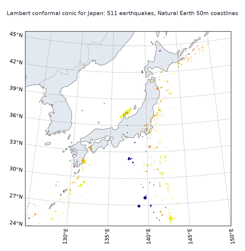
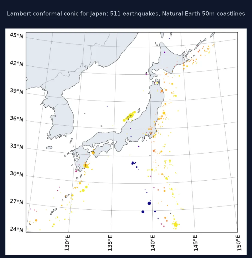
3. Projections compared

Each projection has its own coordinates. Check the units and the width of the world in four common ones:

for name, p in (("PlateCarree", ccrs.PlateCarree()), ("Robinson", ccrs.Robinson()), ("Mollweide", ccrs.Mollweide()),
                ("Orthographic", ccrs.Orthographic(150, 10))):
    w = p.x_limits[1] - p.x_limits[0]
    unit = "degrees" if isinstance(p, ccrs.PlateCarree) else "metres"
    print(f"{name:>12}: x from {p.x_limits[0]:,.0f} to {p.x_limits[1]:,.0f} {unit}")

 PlateCarree: x from -180 to 180 degrees
    Robinson: x from -17,005,833 to 17,005,833 metres
   Mollweide: x from -18,040,096 to 18,040,096 metres
Orthographic: x from -6,378,073 to 6,378,073 metres

PlateCarree works in degrees, while the others work in metres. Robinson spans 34,012 km across and Mollweide 36,080 km. The orthographic globe spans twice the Earth's radius, 12,756 km, because it shows only one hemisphere.

The globe from space

The data used on this page

Every earthquake of magnitude 4.5 or more worldwide in 2024 from the USGS FDSN event service, as CSV. Cartopy downloads the Natural Earth coastlines, land and borders on first use and caches them.

from pathlib import Path

import matplotlib
matplotlib.use("Agg")
import matplotlib.pyplot as plt
import numpy as np
import pandas as pd
import requests
from PIL import Image

Path("data").mkdir(exist_ok=True)
p = Path("data/quakes_m45_2024.csv")
if not p.exists():
    r = requests.get("https://earthquake.usgs.gov/fdsnws/event/1/query", timeout=600,
                     params=dict(format="csv", starttime="2024-01-01", endtime="2025-01-01", minmagnitude=4.5, orderby="time-asc"))
    r.raise_for_status()
    p.write_bytes(r.content)
Q = pd.read_csv(p)
Q = Q[Q["type"] == "earthquake"].reset_index(drop=True)
print(f"{len(Q):,} earthquakes of M4.5+ in 2024")

6,397 earthquakes of M4.5+ in 2024

The catalogue holds 6,397 earthquakes of magnitude 4.5 or more for 2024.

Example 1: the globe from space

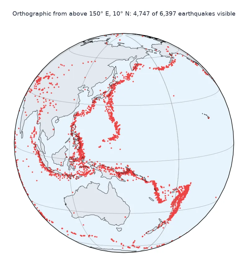
An orthographic projection shows one hemisphere as a globe. Points on the far side are dropped:

ortho = ccrs.Orthographic(central_longitude=150, central_latitude=10)
fig = plt.figure(figsize=(6, 6)); ax3 = plt.axes(projection=ortho); ax3.set_global()
ax3.add_feature(cfeature.LAND, facecolor="#e2e8f0"); ax3.add_feature(cfeature.OCEAN, facecolor="#e8f4fd"); ax3.coastlines(linewidth=0.4)
ax3.gridlines(linewidth=0.3, color="grey")
ax3.scatter(Q.longitude, Q.latitude, s=4, color="#ef4444", transform=ccrs.PlateCarree(), linewidths=0)
fig.savefig("data/cartopy_globe.png", dpi=150, bbox_inches="tight"); plt.close(fig)
xy = ortho.transform_points(ccrs.PlateCarree(), Q.longitude.values, Q.latitude.values)
visible = np.isfinite(xy[:, 0])
print(f"visible from above 150°E, 10°N: {visible.sum():,} of {len(Q):,} earthquakes ({visible.mean():.0%})")

visible from above 150°E, 10°N: 4,747 of 6,397 earthquakes (74%)

Seen from above 150° E, 10° N, 4,747 of the 6,397 earthquakes are on the visible side, 74%, because most of 2024's large earthquakes were around the western Pacific.

Cartopy's coordinate reference objects

Cartopy's central idea is the coordinate reference system object: ccrs.PlateCarree() for plain longitude and latitude, and classes such as Robinson, Mollweide, LambertConformal and Orthographic for projections. A GeoAxes is created in one of them, and every plotting call takes a transform naming the coordinates of its data, which Cartopy reprojects into the axes' projection. When transform is left out, the data is assumed to be already in the axes' coordinates. On a projected map those are metres, so longitude and latitude values of a few hundred become a few hundred metres from the centre, and every point collapses into a dot.

The features come from Natural Earth at three scales, 110m, 50m and 10m, downloaded on first use: the coarse scale suits world maps and the finer ones regional maps. Gridline labels work on most projections with draw_labels=True. Because the output is matplotlib, everything else, from colour bars to annotations and savefig at any resolution, works as usual.

GeoPandas axes, the dateline and set_extent

• GeoPandas on Cartopy axes: gdf.plot(ax=ax, transform=ccrs.PlateCarree()) for data in EPSG:4326, or reproject the GeoDataFrame to the axes' CRS with gdf.to_crs(ax.projection.proj4_init).
• Lines across the dateline: with transform=ccrs.Geodetic() lines follow great circles and cross 180° correctly; PlateCarree draws straight lines in longitude and latitude.
• Offline use: set cartopy.config["data_dir"] to a directory with the Natural Earth files pre-downloaded.
• set_extent: always pass crs=ccrs.PlateCarree() when the extent is in degrees.

Internal links

• Fixing Cartopy points plotted in the wrong place — the transform problem in detail
• Map projections for display explained — choosing a projection
• Great circle vs rhumb line explained — lines on a sphere

FAQ

How do I make a map with Cartopy?

Create axes with plt.axes(projection=ccrs.Robinson()), add ax.coastlines(), and plot data with transform=ccrs.PlateCarree().

What is the difference between projection and transform in Cartopy?

projection is how the map is drawn; transform is the coordinate system of the data being plotted. Longitude and latitude data always takes transform=ccrs.PlateCarree().

How do I centre a Cartopy map on the Pacific?

Use central_longitude=180 in the projection, for example ccrs.Robinson(central_longitude=180).

How do I zoom a Cartopy map to a region?

Call ax.set_extent([lon_min, lon_max, lat_min, lat_max], crs=ccrs.PlateCarree()).