How to Analyse NYC Taxi Trip Records in Python with DuckDB

Problem statement

New York's Taxi & Limousine Commission publishes every yellow-cab trip as monthly Parquet files: pickup and drop-off time, taxi zone, distance, fare and tip. A year is 48,722,602 rows in twelve files of 60–80 MB each — too much to load into pandas comfortably on a laptop, and far more than most questions need. This guide queries the 2025 files where they sit with DuckDB, keeps the trips that belong to the year, counts pickups by zone and maps them, and pulls into pandas only the small tables that answers come from.

Quick answer

Point DuckDB at the Parquet files with read_parquet('data/yellow_tripdata_2025-*.parquet', union_by_name = true), aggregate in SQL, and call .df() on the result. Filter on the pickup time, because each monthly file carries a few trips from other dates.

monthly = con.sql("""
    select date_trunc('month', tpep_pickup_datetime) as month, count(*) as trips
    from trips
    where tpep_pickup_datetime >= '2025-01-01' and tpep_pickup_datetime < '2026-01-01'
    group by 1 order by 1""").df()
print(f"{monthly.trips.sum():,} yellow-taxi trips picked up in 2025")
print(monthly.assign(month=monthly.month.dt.strftime("%b")).set_index("month").trips.to_dict())

48,722,573 yellow-taxi trips picked up in 2025
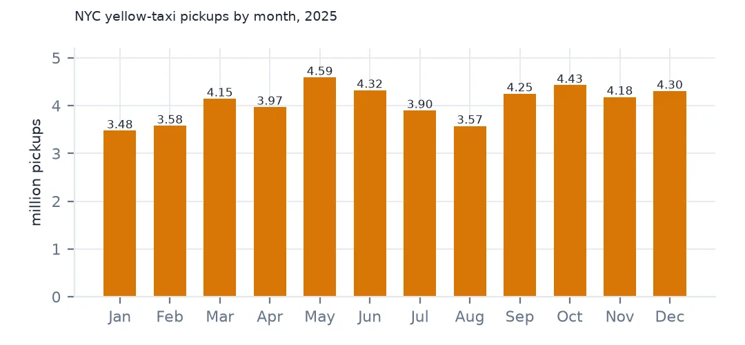
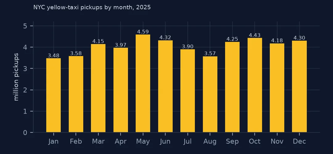
{'Jan': 3475234, 'Feb': 3577542, 'Mar': 4145229, 'Apr': 3970568, 'May': 4591844, 'Jun': 4322949, 'Jul': 3898971, 'Aug': 3574080, 'Sep': 4251019, 'Oct': 4428708, 'Nov': 4181432, 'Dec': 4304997}

There were 48,722,573 yellow-taxi pickups in 2025, from 3,475,234 in January to 4,591,844 in May, the busiest month. The query reads only the one column it needs from each file and finishes in a second.

From twelve files to a pickup map

1. Query the files without loading them

print(con.sql("select count(*) from trips").fetchone()[0], "rows in 12 files")
print(con.sql("describe trips").df()[["column_name", "column_type"]].to_string(index=False))

48722602 rows in 12 files
          column_name column_type
             VendorID     INTEGER
 tpep_pickup_datetime   TIMESTAMP
tpep_dropoff_datetime   TIMESTAMP
      passenger_count      BIGINT
        trip_distance      DOUBLE
           RatecodeID      BIGINT
   store_and_fwd_flag     VARCHAR
         PULocationID     INTEGER
         DOLocationID     INTEGER
         payment_type      BIGINT
          fare_amount      DOUBLE
                extra      DOUBLE
              mta_tax      DOUBLE
           tip_amount      DOUBLE
         tolls_amount      DOUBLE
improvement_surcharge      DOUBLE
         total_amount      DOUBLE
 congestion_surcharge      DOUBLE
          Airport_fee      DOUBLE
   cbd_congestion_fee      DOUBLE

union_by_name lines columns up by name rather than position, which matters because the TLC adds columns over time — cbd_congestion_fee appeared with congestion pricing in January 2025. The count comes from Parquet metadata without reading any rows.

2. Keep trips that belong to the year

out = con.sql("""select count(*) filter (where tpep_pickup_datetime < '2025-01-01') as before,
                        count(*) filter (where tpep_pickup_datetime >= '2026-01-01') as after,
                        min(tpep_pickup_datetime) as earliest from trips""").df()
print(out.to_string(index=False))

 before  after            earliest
     29      0 2007-12-05 18:45:00

Only 29 rows fall outside 2025, the earliest dated December 2007 — meter clocks that were wrong, not trips from 2007. Few as they are, a chart by date would show them as a stray point years before the data starts, so filter by date in every query.

3. Pickups per zone, with names

pu = con.sql("""select PULocationID as LocationID, count(*) as pickups from trips
                where tpep_pickup_datetime >= '2025-01-01' and tpep_pickup_datetime < '2026-01-01' group by 1""").df()
pu = pu.merge(lookup, on="LocationID", how="left")
pu["share"] = pu.pickups / pu.pickups.sum()
print(pu.nlargest(6, "pickups")[["LocationID", "Borough", "Zone", "pickups", "share"]].round(3).to_string(index=False))
print("share of pickups by borough:", pu.groupby("Borough").share.sum().sort_values(ascending=False).round(3).to_dict())

 LocationID   Borough                         Zone  pickups  share
        237 Manhattan        Upper East Side South  2125560  0.044
        161 Manhattan               Midtown Center  2089754  0.043
        132    Queens                  JFK Airport  2062453  0.042
        236 Manhattan        Upper East Side North  1874807  0.038
        186 Manhattan Penn Station/Madison Sq West  1543165  0.032
        230 Manhattan    Times Sq/Theatre District  1516403  0.031
share of pickups by borough: {'Manhattan': 0.858, 'Queens': 0.095, 'Brooklyn': 0.036, 'Bronx': 0.008, 'Unknown': 0.002, 'EWR': 0.0, 'Staten Island': 0.0}

Zones are the only location in the files: the TLC stopped publishing coordinates in 2016. The busiest pickup zone is Upper East Side South, with 2,125,560 pickups (4.4% of the year), and JFK Airport is third. Yellow cabs are a Manhattan service: 85.8% of pickups are there, 9.5% in Queens (mostly the airports) and 0.8% in the Bronx.

4. Map pickups per square kilometre

m = zones.merge(pu[["LocationID", "pickups"]], on="LocationID", how="left").fillna({"pickups": 0})
m["km2"] = m.to_crs(32618).area / 1e6
m["per_km2"] = m.pickups / m.km2
print(f"{len(m)} zones; {(m.pickups < 365).sum()} with fewer than one pickup a day; densest: "
      f"{m.loc[m.per_km2.idxmax(), 'zone']} at {m.per_km2.max():,.0f} pickups per km2 in the year")

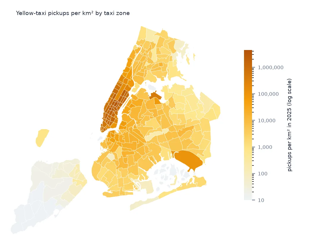
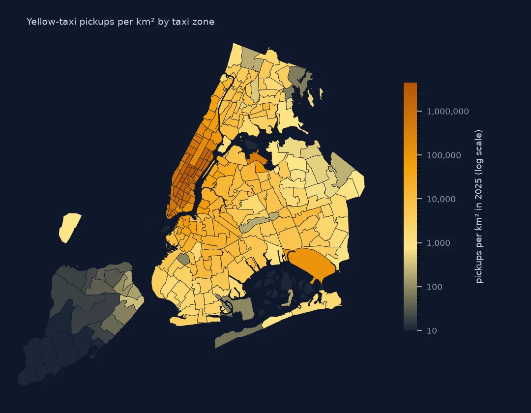
263 zones; 23 with fewer than one pickup a day; densest: Penn Station/Madison Sq West at 4,441,091 pickups per km2 in the year

Dividing by area makes zones of different size comparable. Penn Station/Madison Square West has 4,441,091 pickups per square kilometre over the year; 23 zones average fewer than one pickup a day. The zone shapefile is in New York State Plane (feet), so the area is taken after reprojecting to UTM.

The week and the year

The data used on this page

The NYC Taxi & Limousine Commission's trip record data: the twelve yellow-taxi files for 2025 as Parquet, and the TLC's taxi zones and zone lookup table (saved copies; the TLC reissues them).

from pathlib import Path

import duckdb
import geopandas as gpd
import numpy as np
import pandas as pd
import requests

Path("data").mkdir(exist_ok=True)
TLC = "https://d37ci6vzurychx.cloudfront.net/trip-data/"
FILES = [f"yellow_tripdata_2025-{m:02d}.parquet" for m in range(1, 13)]
for name in FILES:
    if not Path(f"data/{name}").exists():
        with requests.get(TLC + name, stream=True, timeout=600) as r:      # 50-80 MB a month
            r.raise_for_status()
            with open(f"data/{name}", "wb") as f:
                for chunk in r.iter_content(1 << 20):
                    f.write(chunk)
# zones and lookup as the TLC served them on 15 October 2026 (it reissues them; the live copies are
# https://d37ci6vzurychx.cloudfront.net/misc/taxi_zones.zip and .../misc/taxi_zone_lookup.csv)
for name in ["nyc-taxi-zones-2026-10-15.zip", "nyc-taxi-zone-lookup-2026-10-15.csv"]:
    if not Path(f"data/{name}").exists():
        Path(f"data/{name}").write_bytes(requests.get(f"https://data.spatialworkflow.io/{name}", timeout=300).content)
zones = gpd.read_file("zip://data/nyc-taxi-zones-2026-10-15.zip!taxi_zones/taxi_zones.shp")    # EPSG:2263, feet
lookup = pd.read_csv("data/nyc-taxi-zone-lookup-2026-10-15.csv")

con = duckdb.connect()
con.sql("create view trips as select * from read_parquet('data/yellow_tripdata_2025-*.parquet', union_by_name = true)")
print(f"{con.sql('select count(*) from trips').fetchone()[0]:,} rows in trips; {len(zones)} zone polygons, {len(lookup)} lookup rows")

48,722,602 rows in trips; 263 zone polygons, 265 lookup rows

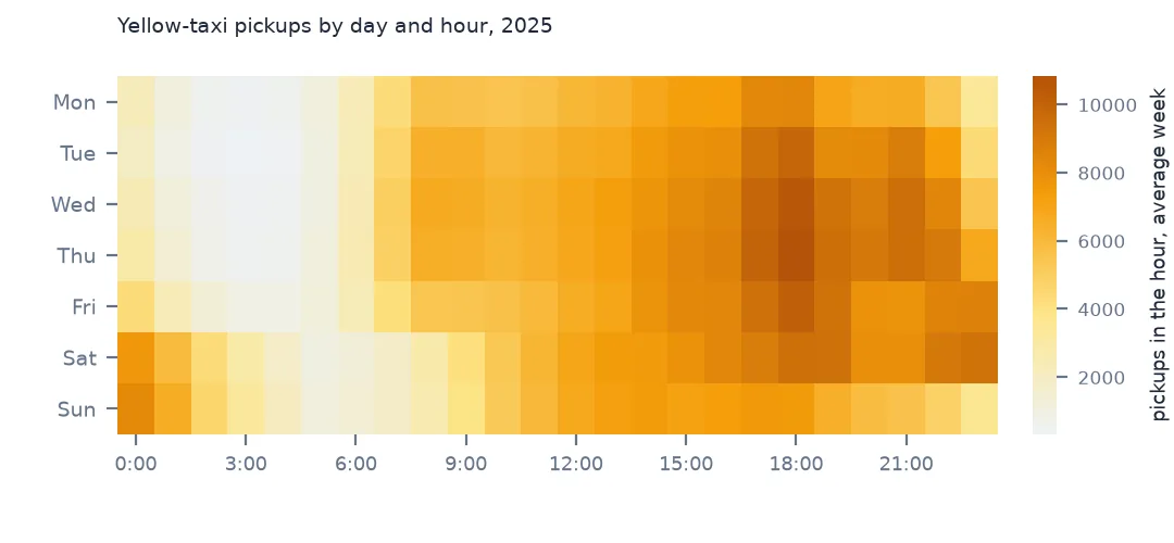
Example 1: the week in one table

wk = con.sql("""select isodow(tpep_pickup_datetime) as dow, hour(tpep_pickup_datetime) as hr, count(*) as n from trips
                where tpep_pickup_datetime >= '2025-01-01' and tpep_pickup_datetime < '2026-01-01' group by 1, 2""").df()
grid = wk.pivot(index="dow", columns="hr", values="n")
DAYS = dict(enumerate(["Mon", "Tue", "Wed", "Thu", "Fri", "Sat", "Sun"], start=1))
(d1, h1), (d0, h0) = grid.stack().idxmax(), grid.stack().idxmin()
print(f"busiest: {DAYS[d1]} {h1}:00, {grid.values.max() / 52:,.0f} pickups in that hour on an average week")
print(f"quietest: {DAYS[d0]} {h0}:00, {grid.values.min() / 52:,.0f} pickups")

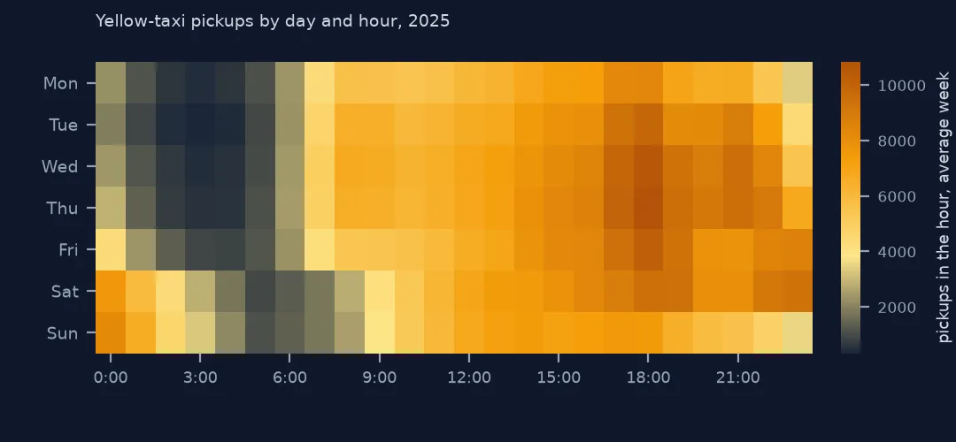
busiest: Thu 18:00, 10,832 pickups in that hour on an average week
quietest: Tue 3:00, 315 pickups

The busiest hour of the week is Thursday at 18:00, with 10,832 pickups on an average week; the quietest is Tuesday at 3:00, with 315.

Example 2: from DuckDB to pandas only when small

day = con.sql("""select cast(tpep_pickup_datetime as date) as d, count(*) as n from trips
                 where tpep_pickup_datetime >= '2025-01-01' and tpep_pickup_datetime < '2026-01-01' group by 1 order by 1""").df()
print(f"{len(day)} days; busiest {day.loc[day.n.idxmax(), 'd']:%a %d %b} ({day.n.max():,}); quietest {day.loc[day.n.idxmin(), 'd']:%a %d %b} ({day.n.min():,})")

365 days; busiest Sat 01 Nov (183,035); quietest Thu 25 Dec (68,111)

The busiest single day was Saturday 1 November (183,035 pickups); the quietest was Christmas Day (68,111).

Why DuckDB suits the trip files

Parquet stores each column separately with statistics for each block, so a query that needs the pickup time and zone reads those two columns and skips the rest; DuckDB runs the aggregation in parallel over the files and returns a small result. The same queries in pandas would first load all twenty columns of every row. The pattern — aggregate in the engine, analyse the result in pandas, join to geometry in GeoPandas — keeps memory proportional to the answer, not the data.

The zones are the TLC's 263 taxi zones, roughly neighbourhoods, plus two codes for unknown and out-of-city locations. Every spatial question about the trips is a question about zones, which sets the resolution of any map.

Before you trust a count

• Payment type 0. About a quarter of 2025 rows have no passenger count, rate code or surcharge fields; they are real trips, but handle them deliberately.
• Files are revised. The TLC occasionally republishes months; record the date you downloaded them.
• Yellow is not all taxis. Green cabs, for-hire vehicles and Uber and Lyft have their own files — the high-volume file is several times larger than the yellow one.
• The unknown and out-of-city zone codes have no polygons; a join to the shapefile drops them silently.

Internal links

• Taxi trip records explained — what each column means
• Taxi zone IDs that do not join — the two zones with no shape
• How to aggregate millions of points into a grid with DuckDB — the same engine on points

FAQ

How many yellow-taxi trips were there in New York in 2025?

48,722,573 pickups dated in 2025 in the TLC's files, before any cleaning.

Do the trip records have coordinates?

Not since mid-2016: only pickup and drop-off taxi zone IDs, joined to the zone shapefile for maps.