
How to Find the Busiest Taxi Routes Between NYC Zones
On this page
Problem statement
Which taxi routes in New York are busiest? With pickups and drop-offs coded to 263 zones, every trip is a zone pair, and a year of yellow-taxi trips fills 54,614 of the 69,169 possible pairs. The busiest are not the famous long trips but short hops between neighbouring zones, and the useful questions are about structure: how few pairs carry most trips, which flows run mainly one way, and how the boroughs exchange trips. This guide answers them for 2025 with one DuckDB aggregation and a little pandas.
Quick answer
Group trips by PULocationID and DOLocationID in DuckDB, drop the unknown zones, and attach zone names from the lookup table. The result is a 54,614-row table that pandas handles easily.
od = con.sql("""select PULocationID as o, DOLocationID as d, count(*) as trips from trips
                where tpep_pickup_datetime >= '2025-01-01' and tpep_pickup_datetime < '2026-01-01'
                  and PULocationID < 264 and DOLocationID < 264 group by 1, 2""").df()
names = lookup.set_index("LocationID").Zone
od["route"] = od.o.map(names) + " -> " + od.d.map(names)
print(f"{len(od):,} zone pairs used out of {263 * 263:,} possible; {od.trips.sum():,} trips")
print(od.nlargest(6, "trips")[["route", "trips"]].to_string(index=False))
54,614 zone pairs used out of 69,169 possible; 48,350,916 trips
route trips
Upper East Side South -> Upper East Side North 302261
Upper East Side North -> Upper East Side South 259469
Upper East Side South -> Upper East Side South 215715
Upper East Side North -> Upper East Side North 197782
Midtown Center -> Upper East Side South 143047
Upper East Side South -> Midtown Center 133753
The busiest route of 2025 was Upper East Side South to Upper East Side North, 302,261 trips, with the reverse second. Four of the top six pairs are within or between those two zones, and the next are between Midtown Center and Upper East Side South: the yellow cab is mostly a short-hop service on Manhattan's East Side.
The shape of the trip table
1. How concentrated the pairs are
s = od.trips.sort_values(ascending=False)
c = s.cumsum() / s.sum()
print(f"top 100 pairs: {c.iloc[99]:.1%} of trips; top 1,000: {c.iloc[999]:.1%}; pairs needed for half: {(c < 0.5).sum() + 1:,}")
print(f"pairs with one trip in the year: {(od.trips == 1).sum():,}")
top 100 pairs: 16.6% of trips; top 1,000: 63.4%; pairs needed for half: 606
pairs with one trip in the year: 4,117
The flows are concentrated: the top 100 pairs carry 16.6% of trips and the top 1,000 carry 63.4%; 606 pairs account for half of all trips. At the other end, 4,117 pairs saw a single trip in the year.
2. Trips that stay in their zone
same = od[od.o == od.d]
print(f"same-zone trips: {same.trips.sum() / od.trips.sum():.1%} of all; busiest: {names[same.loc[same.trips.idxmax(), 'o']]} ({same.trips.max():,})")
same-zone trips: 4.6% of all; busiest: Upper East Side South (215,715)
4.6% of trips start and end in the same zone, most often in Upper East Side South (215,715). These are trips of a few blocks; any analysis of flows between places should report them separately rather than as zero-length lines.
3. One direction or both
a = od.set_index(["o", "d"]).trips
pairs = pd.DataFrame({"ab": a, "ba": a.reindex([(d, o) for o, d in a.index]).values}, index=a.index).dropna()
pairs = pairs[pairs.index.get_level_values(0) < pairs.index.get_level_values(1)]
pairs["total"] = pairs.ab + pairs.ba
big = pairs.nlargest(200, "total")
big["imbalance"] = (big.ab - big.ba).abs() / big.total
top = big.nlargest(3, "imbalance")
for (o, d), r in top.iterrows():
    print(f"{names[o]} -> {names[d]}: {r.ab:,.0f}; back: {r.ba:,.0f}")
print(f"median imbalance among the 200 busiest pairs: {big.imbalance.median():.1%}")
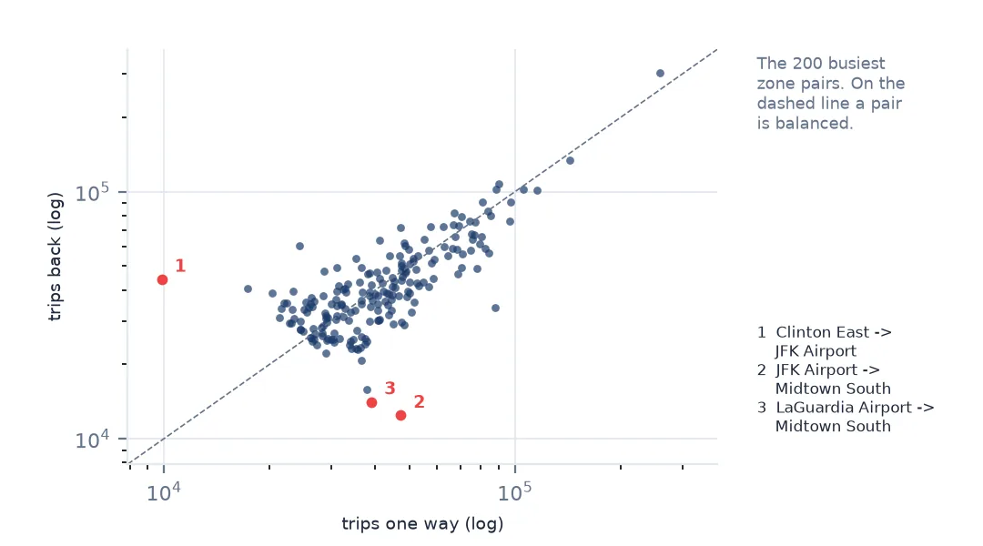
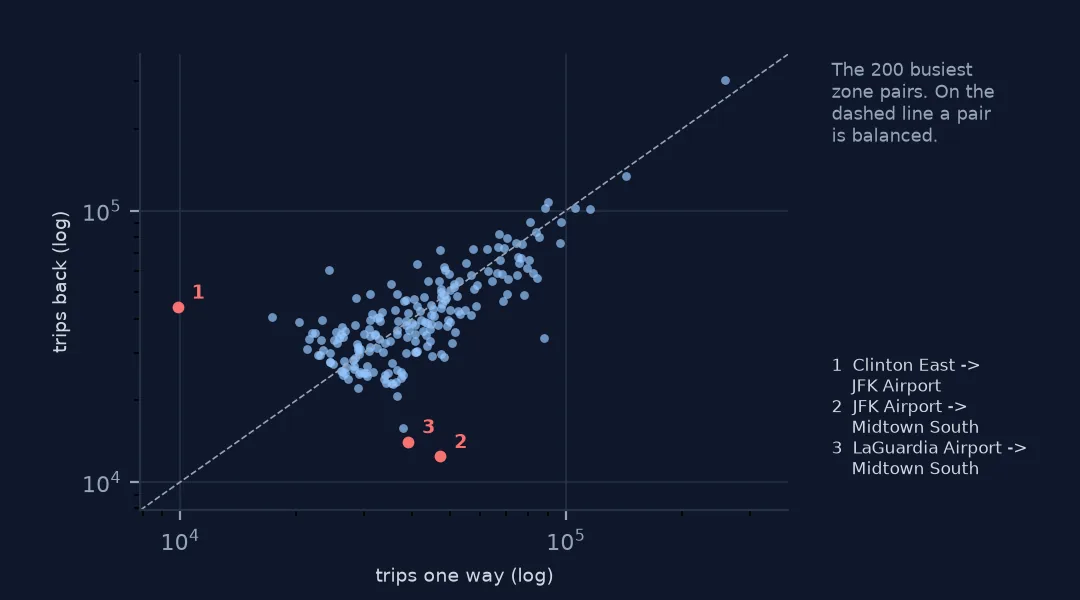
Clinton East -> JFK Airport: 9,869; back: 44,210
JFK Airport -> Midtown South: 47,293; back: 12,449
LaGuardia Airport -> Midtown South: 39,038; back: 14,105
median imbalance among the 200 busiest pairs: 8.4%
Most busy pairs are close to balanced — a median imbalance of 8.4% among the 200 busiest — but the airports are not. 47,293 trips went from JFK to Midtown South and 12,449 back; from Clinton East, 9,869 went to JFK and 44,210 came back. Yellow cabs wait in line at the airports; going there, travellers more often use something else.
4. Borough to borough
bor = lookup.set_index("LocationID").Borough
bm = od.assign(ob=od.o.map(bor), db=od.d.map(bor)).pivot_table(index="ob", columns="db", values="trips", aggfunc="sum", fill_value=0)
print((100 * bm / bm.values.sum()).round(2).to_string())
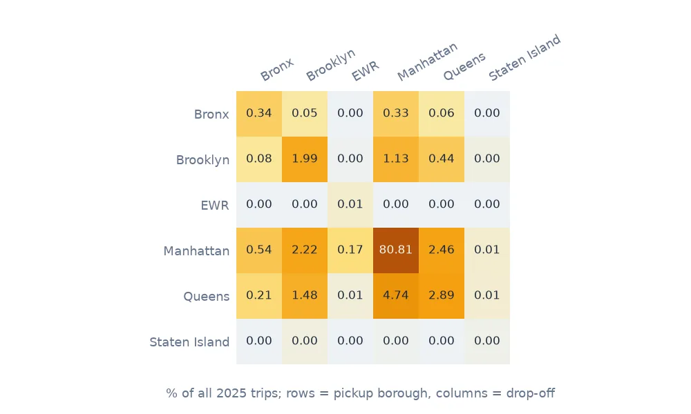
db Bronx Brooklyn EWR Manhattan Queens Staten Island
ob
Bronx 0.34 0.05 0.00 0.33 0.06 0.00
Brooklyn 0.08 1.99 0.00 1.13 0.44 0.00
EWR 0.00 0.00 0.01 0.00 0.00 0.00
Manhattan 0.54 2.22 0.17 80.81 2.46 0.01
Queens 0.21 1.48 0.01 4.74 2.89 0.01
Staten Island 0.00 0.00 0.00 0.00 0.00 0.00
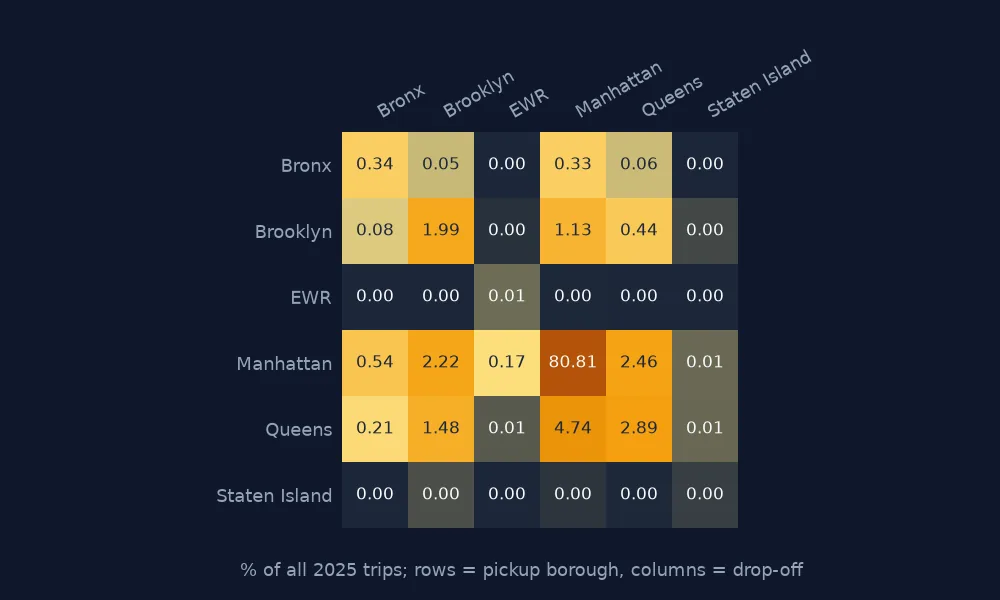
80.81% of all trips start and end in Manhattan. The largest flows involving other boroughs are Queens to Manhattan (4.74%, mostly airport trips) and Manhattan to Queens (2.46%), with Brooklyn to Manhattan at 1.13% and Manhattan to Brooklyn at 2.22%.
Drawing the pairs and timing them
The data used on this page
The NYC Taxi & Limousine Commission's yellow-taxi trip records for 2025 and its taxi zones and lookup table. The two codes for unknown and out-of-city zones are left out of the pairs.
from pathlib import Path

import duckdb
import geopandas as gpd
import numpy as np
import pandas as pd
import requests

Path("data").mkdir(exist_ok=True)
TLC = "https://d37ci6vzurychx.cloudfront.net/trip-data/"
FILES = [f"yellow_tripdata_2025-{m:02d}.parquet" for m in range(1, 13)]
for name in FILES:
    if not Path(f"data/{name}").exists():
        with requests.get(TLC + name, stream=True, timeout=600) as r:      # 50-80 MB a month
            r.raise_for_status()
            with open(f"data/{name}", "wb") as f:
                for chunk in r.iter_content(1 << 20):
                    f.write(chunk)
# zones and lookup as the TLC served them on 15 October 2026 (it reissues them; the live copies are
# https://d37ci6vzurychx.cloudfront.net/misc/taxi_zones.zip and .../misc/taxi_zone_lookup.csv)
for name in ["nyc-taxi-zones-2026-10-15.zip", "nyc-taxi-zone-lookup-2026-10-15.csv"]:
    if not Path(f"data/{name}").exists():
        Path(f"data/{name}").write_bytes(requests.get(f"https://data.spatialworkflow.io/{name}", timeout=300).content)
zones = gpd.read_file("zip://data/nyc-taxi-zones-2026-10-15.zip!taxi_zones/taxi_zones.shp")    # EPSG:2263, feet
lookup = pd.read_csv("data/nyc-taxi-zone-lookup-2026-10-15.csv")

con = duckdb.connect()
con.sql("create view trips as select * from read_parquet('data/yellow_tripdata_2025-*.parquet', union_by_name = true)")
print(f"{con.sql('select count(*) from trips').fetchone()[0]:,} rows in trips; {len(zones)} zone polygons, {len(lookup)} lookup rows")
48,722,602 rows in trips; 263 zone polygons, 265 lookup rows
Example 1: lines between zone centres
cent = zones.set_index("LocationID").geometry.centroid.to_crs(4326)
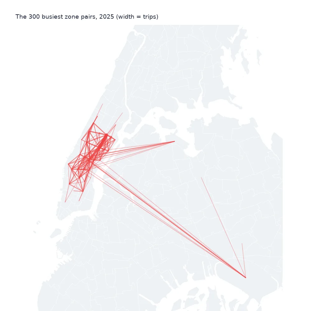
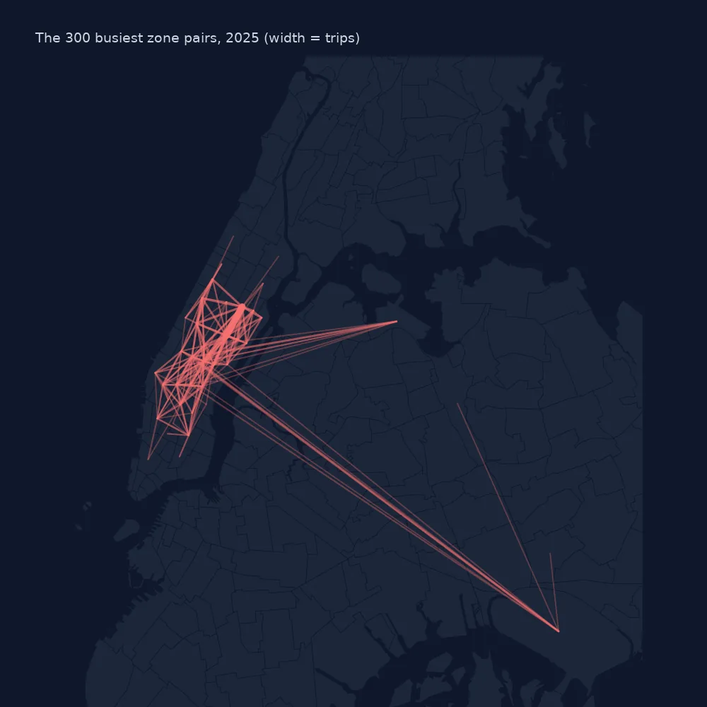
top_lines = od[od.o != od.d].nlargest(300, "trips")
print(f"300 busiest pairs between different zones carry {top_lines.trips.sum() / od.trips.sum():.1%} of trips; "
      f"median straight-line length {top_lines.apply(lambda r: cent[r.o].distance(cent[r.d]), axis=1).median() * 111:.1f} km (approximate)")
300 busiest pairs between different zones carry 32.1% of trips; median straight-line length 1.8 km (approximate)
The 300 busiest pairs between different zones carry 32.1% of trips, and their median length between zone centres is about 1.8 km. Lines that short are best drawn on a zoomed map of Manhattan, with line width proportional to trips, or the airports' longer lines dominate the picture.
Example 2: the busiest pair by hour
o0, d0 = od[od.o != od.d].nlargest(1, "trips")[["o", "d"]].iloc[0]
h = con.sql(f"""select hour(tpep_pickup_datetime) as h, count(*) as n from trips
               where PULocationID = {o0} and DOLocationID = {d0} group by 1 order by 1""").df().set_index("h").n
print(f"{names[o0]} -> {names[d0]}: peak hour {h.idxmax()}:00 ({h.max():,} trips over the year), quietest {h.idxmin()}:00 ({h.min():,})")
Upper East Side South -> Upper East Side North: peak hour 14:00 (26,949 trips over the year), quietest 4:00 (85)
The busiest route peaks at 14:00, with 26,949 trips in that hour across the year, and falls to 85 at 4:00 — an afternoon errand route rather than a commute.
Zone pairs as an origin-destination matrix
The table of zone pairs is an origin-destination matrix stored in long form: one row per pair with trips, rather than a 263 × 263 grid that would be mostly empty. Long form keeps only the pairs that occurred and joins easily to names, geometry or travel times; the general guide to OD matrices covers pivoting and reading it.
Taxi flows describe taxi demand, not travel demand. Many trips between the Upper East Side and Midtown are made by subway or bus; yellow cabs win where the subway is awkward (crosstown, the East Side before the Second Avenue line) and where luggage is involved. A busiest-route table shows where the taxi is the chosen mode.
Things to decide before ranking routes
- Direction. A→B and B→A are separate rows; add them for corridor totals, keep them apart for asymmetry.
- Unknown zones. The unknown and out-of-city codes are dropped here; with them, airport and out-of-city flows look different.
- Zone size. Large zones hold more internal trips; compare internal trips by area or population before ranking.
- Ride-hail. Uber and Lyft carry several times more trips with a different geography; a route table from yellow cabs alone describes only part of the market.
Internal links
- How to build and read an origin-destination matrix — the general method
- How to build desire lines — drawing pairs as lines
- Taxi zone IDs that do not join — why two IDs are dropped here
FAQ
What is the busiest taxi route in New York?
In 2025, Upper East Side South to Upper East Side North, with 302,261 yellow-taxi trips.
How many zone pairs carry half of all taxi trips?
606 of the 54,614 pairs used in 2025.