How to Measure the Effect of Congestion Pricing with Taxi Trip Data

Problem statement

On 5 January 2025 New York began charging vehicles that enter Manhattan below 60th Street — the first congestion pricing scheme in the United States. Whether it made traffic faster is a spatial before-and-after question, and taxi trip records can answer part of it: every trip has a start and end time, a metered distance and its zones, for the same months before and after the change. The work is in the comparison — which zones are inside, which trips and hours to compare, and what to use as a control. This guide derives the zone from the new fee column, compares weekday daytime taxi speeds inside it for January–June 2024 and 2025, and checks the result against Manhattan outside the zone.

Quick answer

Find the zones where trips that start and end in the same zone are charged the cbd_congestion_fee, then compare the ratio of total distance to total time for trips wholly inside those zones, on the same weekday hours and months of both years. For yellow taxis inside the zone, speed rose by 2.5%.

crz = con.sql("""select PULocationID as LocationID, avg((cbd_congestion_fee > 0)::int) as f from y25
                 where PULocationID = DOLocationID and payment_type <> 0 group by 1 having count(*) > 200""").df()
crz_ids = crz[(crz.f > 0.5) & (crz.LocationID < 264)].LocationID.tolist()    # 264 is 'unknown', not a place
sp = con.sql(f"""
    select year(tpep_pickup_datetime) as yr, count(*) as trips, sum(trip_distance) / sum(epoch(tpep_dropoff_datetime - tpep_pickup_datetime) / 3600) as mph
    from h1 where year(tpep_pickup_datetime) in (2024, 2025) and PULocationID in {tuple(crz_ids)} and DOLocationID in {tuple(crz_ids)}
      and isodow(tpep_pickup_datetime) <= 5 and hour(tpep_pickup_datetime) between 7 and 18
      and trip_distance between 0.5 and 10 and epoch(tpep_dropoff_datetime - tpep_pickup_datetime) between 72 and 7200
    group by 1 order by 1""").df()
print(f"{len(crz_ids)} zones inside the congestion relief zone")
print(sp.round(2).to_string(index=False))
print(f"change in speed, Jan-Jun 2025 against 2024: {sp.mph.iloc[1] / sp.mph.iloc[0] - 1:+.1%}")

38 zones inside the congestion relief zone
  yr   trips  mph
2024 3390467 7.31
2025 3699932 7.50
change in speed, Jan-Jun 2025 against 2024: +2.5%

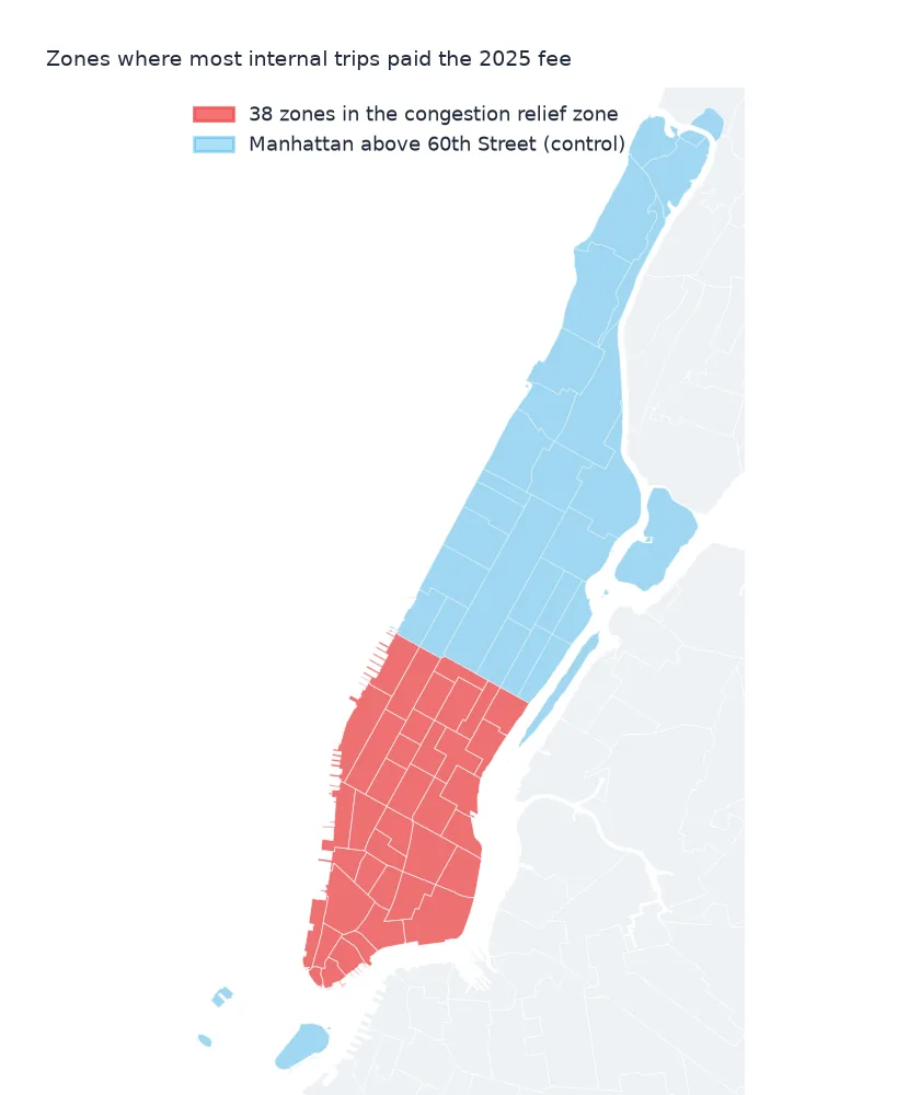
38 taxi zones lie inside the congestion relief zone. Weekday daytime taxi trips within it averaged 7.31 mph in January–June 2024 and 7.50 mph in the same months of 2025. Taxis there also made more of these trips in 2025, not fewer: 3,699,932 against 3,390,467.

Building a fair before-and-after

1. Find the zone from the fee

print("zones by share of internal trips charged:", pd.cut(crz[crz.LocationID < 264].f, [-0.01, 0.05, 0.5, 1], labels=['under 5%', '5-50%', 'over 50%']).value_counts().sort_index().to_dict())
z = lookup.set_index("LocationID").loc[crz_ids]
print("examples:", z.Zone.head(4).tolist(), "| boroughs:", z.Borough.unique().tolist())

zones by share of internal trips charged: {'under 5%': 108, '5-50%': 6, 'over 50%': 38}
examples: ['Alphabet City', 'Battery Park', 'Battery Park City', 'Chinatown'] | boroughs: ['Manhattan']

The fee splits the zones cleanly: 38 zones charge more than half of their internal trips, 108 charge under 5%, and only 6 fall between, along the 60th Street boundary and the highways the scheme exempts. Deriving the zone from the data avoids hand-typing a list of IDs, and it is the definition the meters actually applied.

2. Same months, same hours, both years

n = con.sql(f"""select year(tpep_pickup_datetime) as yr, month(tpep_pickup_datetime) as m, count(*) as n from h1
                where tpep_pickup_datetime >= '2024-01-01' and month(tpep_pickup_datetime) <= 6 group by 1, 2""").df()
t = n.pivot(index="m", columns="yr", values="n")
print((t[2025] / t[2024] - 1).round(3).to_dict(), "change in all yellow trips, by month")

{1: 0.172, 2: 0.19, 3: 0.157, 4: 0.13, 5: 0.233, 6: 0.221} change in all yellow trips, by month

All yellow trips grew by 13% to 23% month on month from 2024 to 2025. Growth like that, citywide, changes how busy the streets are on its own; it is why a control area is needed below.

3. Trips that touch the zone

touch = con.sql(f"""select year(tpep_pickup_datetime) as yr,
        avg((PULocationID in {tuple(crz_ids)} or DOLocationID in {tuple(crz_ids)})::int) as touches,
        avg((PULocationID in {tuple(crz_ids)} and DOLocationID in {tuple(crz_ids)})::int) as inside
        from h1 where year(tpep_pickup_datetime) in (2024, 2025) and month(tpep_pickup_datetime) <= 6 group by 1 order by 1""").df()
print(touch.round(3).to_string(index=False))

  yr  touches  inside
2024    0.730   0.414
2025    0.715   0.412

The share of yellow trips that start or end in the zone barely moved, from 0.730 to 0.715, and the share wholly inside it from 0.414 to 0.412. Taxis pay the fee per trip, passed on to the passenger, and it did not change where people took cabs.

4. Speed by hour, before and after

hr = con.sql(f"""
    select year(tpep_pickup_datetime) as yr, hour(tpep_pickup_datetime) as h,
           sum(trip_distance) / sum(epoch(tpep_dropoff_datetime - tpep_pickup_datetime) / 3600) as mph
    from h1 where year(tpep_pickup_datetime) in (2024, 2025) and PULocationID in {tuple(crz_ids)} and DOLocationID in {tuple(crz_ids)} and isodow(tpep_pickup_datetime) <= 5
      and trip_distance between 0.5 and 10 and epoch(tpep_dropoff_datetime - tpep_pickup_datetime) between 72 and 7200
    group by 1, 2""").df().pivot(index="h", columns="yr", values="mph")
gain = hr[2025] / hr[2024] - 1
print(f"largest gain {gain.max():+.1%} at {gain.idxmax()}:00; smallest {gain.min():+.1%} at {gain.idxmin()}:00")
print("weekday speed inside the zone, mph:", hr.loc[[8, 13, 18, 22]].round(2).to_dict("index"))

largest gain +3.1% at 17:00; smallest +0.2% at 6:00
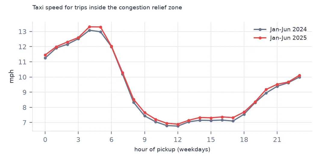
weekday speed inside the zone, mph: {8: {2024: 8.33, 2025: 8.53}, 13: {2024: 7.04, 2025: 7.15}, 18: {2024: 7.55, 2025: 7.69}, 22: {2024: 9.62, 2025: 9.67}}

Speeds rose at every hour, by most in the evening peak (+3.1% at 17:00) and least early in the morning (+0.2% at 6:00), when there is little traffic to remove. Even after the change, midday taxis in the zone average about 7 mph.

A control area and the fee itself

The data used on this page

The NYC Taxi & Limousine Commission's yellow-taxi trip records for January–June 2024 and all of 2025, and its taxi zones. Congestion pricing in Manhattan below 60th Street began on 5 January 2025; taxi trips that start, end or pass through the zone pay a per-trip fee recorded in cbd_congestion_fee.

from pathlib import Path

import duckdb
import geopandas as gpd
import numpy as np
import pandas as pd
import requests

Path("data").mkdir(exist_ok=True)
TLC = "https://d37ci6vzurychx.cloudfront.net/trip-data/"
FILES = [f"yellow_tripdata_{y}-{m:02d}.parquet" for y, ms in [(2024, range(1, 7)), (2025, range(1, 13))] for m in ms]
for name in FILES:
    if not Path(f"data/{name}").exists():
        with requests.get(TLC + name, stream=True, timeout=600) as r:      # 50-80 MB a month
            r.raise_for_status()
            with open(f"data/{name}", "wb") as f:
                for chunk in r.iter_content(1 << 20):
                    f.write(chunk)
# zones and lookup as the TLC served them on 15 October 2026 (it reissues them; the live copies are
# https://d37ci6vzurychx.cloudfront.net/misc/taxi_zones.zip and .../misc/taxi_zone_lookup.csv)
for name in ["nyc-taxi-zones-2026-10-15.zip", "nyc-taxi-zone-lookup-2026-10-15.csv"]:
    if not Path(f"data/{name}").exists():
        Path(f"data/{name}").write_bytes(requests.get(f"https://data.spatialworkflow.io/{name}", timeout=300).content)
zones = gpd.read_file("zip://data/nyc-taxi-zones-2026-10-15.zip!taxi_zones/taxi_zones.shp")    # EPSG:2263, feet
lookup = pd.read_csv("data/nyc-taxi-zone-lookup-2026-10-15.csv")

con = duckdb.connect()
con.sql("create view h1 as select * from read_parquet(['data/yellow_tripdata_2024-0[1-6].parquet', 'data/yellow_tripdata_2025-0[1-6].parquet'], union_by_name = true)")
con.sql("create view y25 as select * from read_parquet('data/yellow_tripdata_2025-*.parquet', union_by_name = true)")
con.register("lookup_df", lookup)
print(f"{con.sql('select count(*) from h1').fetchone()[0]:,} rows in h1; {len(zones)} zone polygons, {len(lookup)} lookup rows")

44,415,477 rows in h1; 263 zone polygons, 265 lookup rows

Example 1: outside the zone as a control

out = con.sql(f"""
    select year(tpep_pickup_datetime) as yr, sum(trip_distance) / sum(epoch(tpep_dropoff_datetime - tpep_pickup_datetime) / 3600) as mph
    from h1 where year(tpep_pickup_datetime) in (2024, 2025) and PULocationID not in {tuple(crz_ids)} and DOLocationID not in {tuple(crz_ids)}
      and PULocationID in (select LocationID from lookup_df where Borough = 'Manhattan')
      and DOLocationID in (select LocationID from lookup_df where Borough = 'Manhattan')
      and isodow(tpep_pickup_datetime) <= 5 and hour(tpep_pickup_datetime) between 7 and 18
      and trip_distance between 0.5 and 10 and epoch(tpep_dropoff_datetime - tpep_pickup_datetime) between 72 and 7200
    group by 1 order by 1""").df()
print(f"Manhattan above 60th Street, weekday daytime: {out.mph.iloc[0]:.2f} -> {out.mph.iloc[1]:.2f} mph ({out.mph.iloc[1] / out.mph.iloc[0] - 1:+.1%})")

Manhattan above 60th Street, weekday daytime: 8.50 -> 8.47 mph (-0.3%)

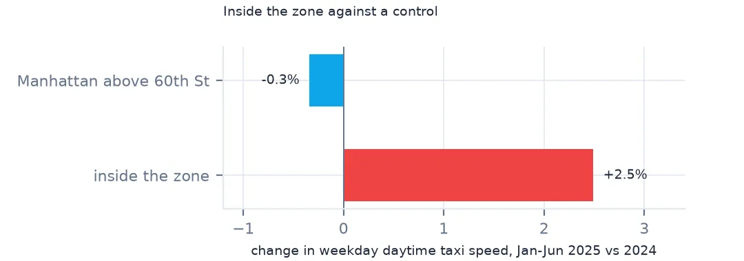
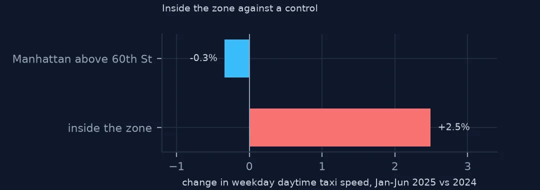
Manhattan above 60th Street, outside the zone, is the natural control: same borough, same cabs, same months, no charge. There, weekday daytime speed fell slightly, from 8.50 to 8.47 mph (−0.3%). The difference between +2.5% inside and −0.3% outside is the part of the change that can be put down to the zone — a difference-in-differences of nearly three points, small but in the expected direction.

Example 2: the fee through the year

fee = con.sql("""select month(tpep_pickup_datetime) as m, avg((cbd_congestion_fee > 0)::int) as charged,
                 sum((cbd_congestion_fee < 0)::int) as reversed from y25 where year(tpep_pickup_datetime) = 2025 group by 1 order by 1""").df()
print("share of 2025 trips charged, by month:", fee.set_index("m").charged.round(3).to_dict())
print(f"rows with a negative fee (refunds and reversals): {int(fee.reversed.sum()):,}")

share of 2025 trips charged, by month: {1: 0.646, 2: 0.727, 3: 0.727, 4: 0.723, 5: 0.715, 6: 0.723, 7: 0.727, 8: 0.719, 9: 0.725, 10: 0.724, 11: 0.721, 12: 0.711}
rows with a negative fee (refunds and reversals): 509,663

In January 64.6% of trips were charged — the fee started on the 5th — and from February about 72% each month. 509,663 rows carry a negative fee, reversals of a charge, so count trips with cbd_congestion_fee > 0 rather than summing the column.

What taxi speeds can and cannot show

A taxi trip's average speed includes everything: waiting at lights, turning, stopping to let a passenger out. It is a measure of how fast a door-to-door journey is, not of traffic flow on a road. For a before-and-after comparison that is fine as long as both periods are measured the same way — same zones, same hours, same weekdays, same trip-length filter — which is what the queries enforce.

What the comparison cannot do is isolate the scheme from everything else that changed between 2024 and 2025: more taxi trips, the economy, roadworks, weather. The control area takes out what affected all of Manhattan alike; it cannot take out what happened only below 60th Street. Official evaluations use road sensors, bus GPS and many more vehicles, and they are the place to go for the policy verdict. What taxi data gives you is an independent check that anyone can run.

Choices that move the answer

• Ratio of sums, not mean of ratios. Total distance over total time weights long trips by their length; averaging per-trip speeds lets very short trips dominate. See how to calculate speeds from taxi trips.
• Trips through the zone. A trip from Brooklyn to the Upper West Side may cross the zone and pay the fee while starting and ending outside it. Comparing trips wholly inside avoids that.
• Payment type 0. Flex-fare rows are kept in these speed queries; their distances and times are recorded the same way.
• Calendar effects. January 2025 began on a Wednesday and 2024 on a Monday; comparing whole months is close enough for speeds, not for daily counts.

Internal links

• How to calculate traffic speeds by hour from taxi trips — the speed method
• Taxi trip records explained — the fee and surcharge columns
• How to analyse UK traffic count data — traffic measured by counters instead

FAQ

Did congestion pricing make traffic faster in Manhattan?

For yellow taxis inside the zone, weekday daytime speeds were 2.5% higher in January–June 2025 than in 2024, while Manhattan above 60th Street was 0.3% slower.

Which taxi zones are in the congestion relief zone?

The 38 zones where most trips that start and end in the zone pay the fee, all in Manhattan; step 1 derives them from the 2025 records.