
How to Read a GBFS Bike-Share Feed in Python
On this page
Problem statement
Almost every bike-share system in the world publishes its live state in the General Bikeshare Feed Specification (GBFS): a set of small JSON files, refreshed every minute, that say where the stations are, how many bikes and free docks each has right now, and where the bikes outside a dock are parked. Apps read them; so can anyone with requests. The files are simple, but they are a set, and reading one alone gives wrong answers — the status file has no coordinates, the station file has no counts, and the ids in both differ from the ids in the same operator's trip files.
This page reads Capital Bikeshare's feed in Washington, D.C. from its discovery file down, joins stations to their status and regions, looks at the parked e-bikes, and connects the feed to the historical trip files.
Quick answer
Load station_information and station_status, merge them on station_id, keep the stations that are installed and renting, and count:
info = pd.DataFrame(load("station_information")["data"]["stations"])
status = pd.DataFrame(load("station_status")["data"]["stations"])
st = info.merge(status, on="station_id", validate="one_to_one")
live = st[(st.is_installed == 1) & (st.is_renting == 1)]
print(f"{len(st)} stations, {len(live)} renting; snapshot {stamp('station_status'):%Y-%m-%d %H:%M %Z}")
print(f"empty: {(live.num_bikes_available == 0).sum()}   full: {(live.num_docks_available == 0).sum()}   "
      f"bikes available: {live.num_bikes_available.sum():,} ({live.num_ebikes_available.sum():,} e-bikes)")
868 stations, 863 renting; snapshot 2026-10-15 08:03 EDT
empty: 41 full: 30 bikes available: 5,839 (1,823 e-bikes)
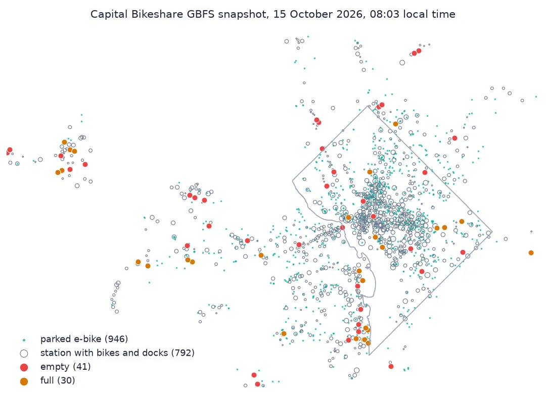
At 08:03 on a Thursday in October 2026, 41 of 863 renting stations had no bike to rent and 30 had no free dock to return one to. 5,839 bikes were waiting in docks, 1,823 of them e-bikes. The validate="one_to_one" in the merge is not decoration: if a station appeared twice in either file, the counts would double silently.
From the discovery file to a joined snapshot
1. Start from the auto-discovery file
A GBFS system publishes one root file, gbfs.json, that lists every other feed and its URL. Read it rather than hard-coding the URLs; operators move them (Capital Bikeshare's root lives on its own domain, the feeds on Lyft's):
gbfs = load("gbfs")
print(f"version {gbfs['version']}, ttl {gbfs['ttl']} s")
for f in gbfs["data"]["en"]["feeds"]:
    print(f"  {f['name']:22s} {f['url'].rsplit('/', 1)[-1]}")
version 2.3, ttl 60 s
gbfs gbfs.json
system_information system_information.json
station_information station_information.json
station_status station_status.json
free_bike_status free_bike_status.json
system_hours system_hours.json
system_calendar system_calendar.json
system_regions system_regions.json
system_pricing_plans system_pricing_plans.json
system_alerts system_alerts.json
gbfs_versions gbfs_versions.json
vehicle_types vehicle_types.json
Twelve feeds, each with a time to live of 60 seconds — a client should not ask again sooner. Version 2.3 is what this system serves; GBFS 3.0 renames several fields (free_bike_status becomes vehicle_status), so check version before parsing.
2. Stations and regions
regions = pd.DataFrame(load("system_regions")["data"]["regions"]).set_index("region_id").name
info["region"] = info.region_id.map(regions).fillna("no region")
print(info.groupby("region").agg(stations=("station_id", "size"), docks=("capacity", "sum"))
      .sort_values("stations", ascending=False).to_string())
print(f"station_id looks like {info.station_id.iloc[0]!r}; short_name like {info.short_name.iloc[0]!r}")
stations docks
region
Washington, DC 397 8065
Arlington, VA 111 1572
Fairfax, VA 106 1343
Alexandria, VA 71 1075
Montgomery County, MD (South) 56 873
no region 56 799
Prince George's County 38 573
Montgomery County, MD (North) 23 364
Falls Church, VA 10 119
station_id looks like '0824ea2c-1f3f-11e7-bf6b-3863bb334450'; short_name like '31014'
The system spans eight jurisdictions and three states. 397 of its 868 stations are in the District itself; 56, with 799 docks between them, carry no region at all, so any table by region needs that row. The station id is a UUID. The number riders and the trip files use is the short_name.
3. What a station's status says
st["fill"] = st.num_bikes_available / (st.num_bikes_available + st.num_docks_available)
age = (stamp("station_status") - pd.to_datetime(st.last_reported, unit="s", utc=True)).dt.total_seconds() / 60
print(f"not installed {(st.is_installed == 0).sum()}, installed but not renting {((st.is_installed == 1) & (st.is_renting == 0)).sum()}")
print(f"disabled bikes {st.num_bikes_disabled.sum():,}, disabled docks {st.num_docks_disabled.sum():,}")
print(f"last report older than an hour: {(age > 60).sum()} stations; median age {age.median():.1f} min")
gap = st.capacity - (st.num_bikes_available + st.num_docks_available + st.num_bikes_disabled + st.num_docks_disabled)
print("capacity minus everything counted, stations:", gap.value_counts().sort_index().to_dict())
not installed 0, installed but not renting 5
disabled bikes 573, disabled docks 42
last report older than an hour: 4 stations; median age 0.8 min
capacity minus everything counted, stations: {-2: 2, -1: 19, 0: 743, 1: 89, 2: 11, 3: 2, 4: 1, 7: 1}
A station that is listed is not necessarily usable. Five were installed but not renting. 573 bikes sat in docks marked disabled — broken or awaiting service, invisible to riders but taking up a dock. Four stations had not reported for over an hour, so their counts were stale; the median station had reported within the last minute. And capacity is not the sum of what a station reports: at 89 stations it is one more, at 21 it is one or two fewer. Use the reported counts, not capacity, when asking how full a station is.
4. Free-floating e-bikes
bikes = pd.DataFrame(load("free_bike_status")["data"]["bikes"])
types = pd.DataFrame(load("vehicle_types")["data"]["vehicle_types"]).set_index("vehicle_type_id")
print(bikes.vehicle_type_id.map(types.propulsion_type).value_counts().to_string())
print(f"{len(bikes)} bikes outside a dock; range: median {bikes.current_range_meters.median() / 1000:.1f} km, "
      f"under 5 km: {(bikes.current_range_meters < 5000).sum()}")
print(f"coordinate decimals, median: {bikes.lat.astype(str).str.split('.').str[1].str.len().median():.0f}")
vehicle_type_id
electric_assist 946
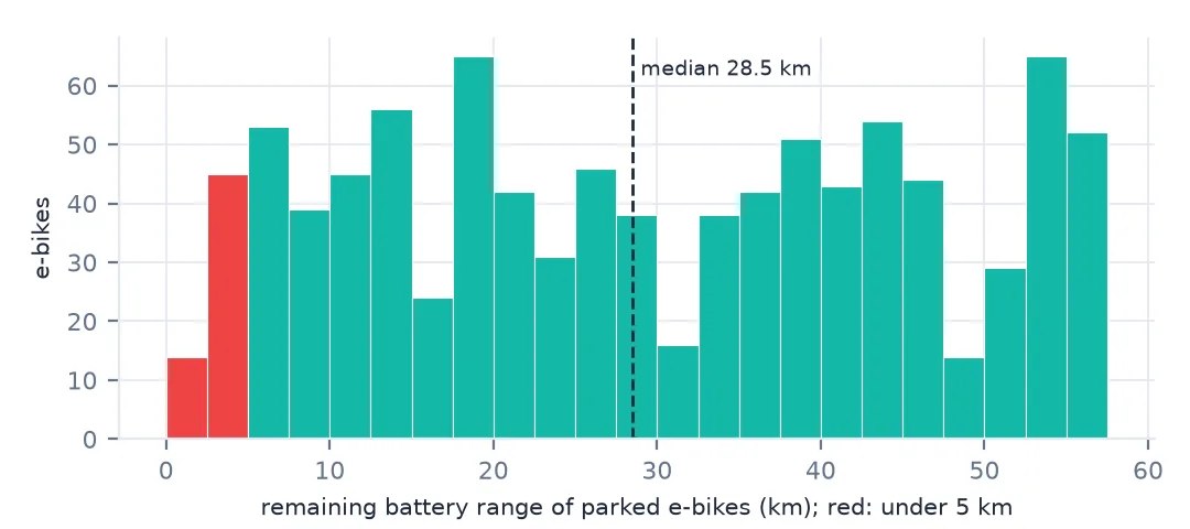
946 bikes outside a dock; range: median 28.5 km, under 5 km: 59
coordinate decimals, median: 9
Every one of the 946 bikes parked outside a dock is an e-bike, with a battery range attached: a median of 28.5 km, and 59 with under 5 km left. Their coordinates have nine decimal places — in the trip files the same kind of location is rounded to two.
5. Join the feed to the trip files
The feed and the trip files describe the same stations, so a historical analysis can take station locations and capacities from the feed. The key has to be the right one:
trip_ids = pd.read_csv(zipfile.ZipFile("data/202512-capitalbikeshare-tripdata.zip").open("202512-capitalbikeshare-tripdata.csv"),
                       usecols=["start_station_id"]).start_station_id.dropna().astype(int).unique()
short = pd.to_numeric(info.short_name, errors="coerce")
print(f"trip-file station ids found as GBFS station_id: {np.isin(trip_ids.astype(str), info.station_id).sum()}, "
      f"as short_name: {np.isin(trip_ids, short).sum()} of {len(trip_ids)}")
trip-file station ids found as GBFS station_id: 0, as short_name: 812 of 815
None of December 2025's station ids appear as a GBFS station_id; 812 of 815 appear as short_name. The three left over are no longer in the feed, which is the other reason to keep a dated copy of station_information alongside any trip analysis.
Empty stations and parked e-bikes
The data used on this page
Capital Bikeshare's public GBFS feed (General Bikeshare Feed Specification, version 2.3, operated by Lyft), and the December 2025 trip file from the operator's system data. The feed changes every minute: the setup saves one copy of every file it lists, and every block on this page reads that copy, so the numbers describe one moment — the snapshot of 15 October 2026 shown in the output. A new run saves a new moment.
from pathlib import Path
import json
import time
import zipfile

import numpy as np
import pandas as pd
import requests

SNAP = Path("data/gbfs")
SNAP.mkdir(parents=True, exist_ok=True)
if not (SNAP / "gbfs.json").exists():
    root = requests.get("https://gbfs.capitalbikeshare.com/gbfs/2.3/gbfs.json", timeout=60).json()
    (SNAP / "gbfs.json").write_text(json.dumps(root))
    for feed in root["data"]["en"]["feeds"]:
        (SNAP / f"{feed['name']}.json").write_text(requests.get(feed["url"], timeout=60).text)
        time.sleep(0.5)
f = Path("data/202512-capitalbikeshare-tripdata.zip")
if not f.exists():
    f.write_bytes(requests.get(f"https://s3.amazonaws.com/capitalbikeshare-data/{f.name}", timeout=600).content)


def load(name):
    return json.loads((SNAP / f"{name}.json").read_text())


def stamp(name):
    return pd.Timestamp(load(name)["last_updated"], unit="s", tz="UTC").tz_convert("America/New_York")


print(sorted(p.stem for p in SNAP.glob("*.json")))
['free_bike_status', 'gbfs', 'gbfs_versions', 'station_information', 'station_status', 'system_alerts', 'system_calendar', 'system_hours', 'system_information', 'system_pricing_plans', 'system_regions', 'vehicle_types']
Example 1: which stations are empty, and where
live = st[(st.is_installed == 1) & (st.is_renting == 1)].copy()
live["region"] = live.region_id.map(regions).fillna("no region")
live["state"] = np.select([live.num_bikes_available == 0, live.num_docks_available == 0], ["empty", "full"], "in between")
print(pd.crosstab(live.region, live.state, margins=True).to_string())
state empty full in between All
region
Alexandria, VA 4 7 60 71
Arlington, VA 3 2 105 110
Fairfax, VA 8 9 86 103
Falls Church, VA 1 1 8 10
Montgomery County, MD (North) 3 0 20 23
Montgomery County, MD (South) 8 1 47 56
Prince George's County 2 1 35 38
Washington, DC 5 7 385 397
no region 7 2 46 55
All 41 30 792 863
The District, where rebalancing trucks are busiest, had 5 empty stations of 397. The suburbs fared worse on that morning: 8 of 56 stations in southern Montgomery County and 8 of 103 in Fairfax were empty. One snapshot is one moment — the same table at 6 p.m. would look different — but it is the moment a rider at 8 a.m. sees.
Example 2: how far parked e-bikes are from a dock
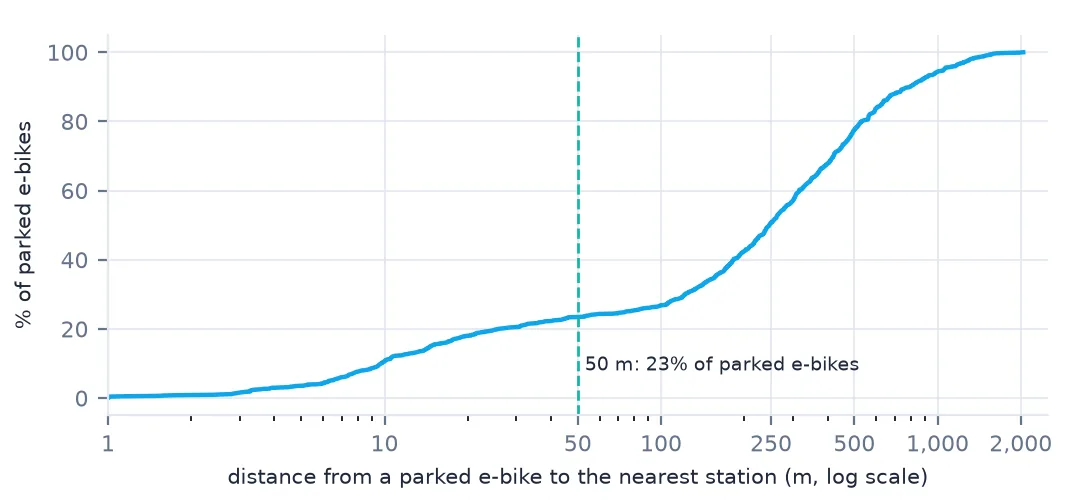
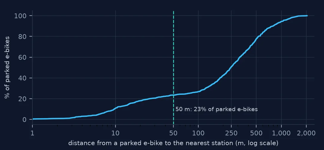
The parked e-bikes are where trips ended without a dock. Their distance from the nearest station shows how far they stray:
def metres(lat1, lon1, lat2, lon2):
    lat1, lon1, lat2, lon2 = map(np.radians, (lat1, lon1, lat2, lon2))
    a = np.sin((lat2 - lat1) / 2) ** 2 + np.cos(lat1) * np.cos(lat2) * np.sin((lon2 - lon1) / 2) ** 2
    return 2 * 6_371_008.8 * np.arcsin(np.sqrt(a))


d = metres(bikes.lat.values[:, None], bikes.lon.values[:, None], info.lat.values[None, :], info.lon.values[None, :])
bikes["to_dock_m"] = d.min(axis=1)
print(bikes.to_dock_m.describe(percentiles=[0.1, 0.25, 0.5, 0.75, 0.9]).round(0).to_string())
print(f"within 50 m of a station: {(bikes.to_dock_m <= 50).mean():.0%}")
count 946.0
mean 335.0
std 337.0
min 0.0
10% 10.0
25% 76.0
50% 247.0
75% 477.0
90% 794.0
max 2040.0
within 50 m of a station: 23%
A median parked e-bike is 247 m from the nearest station, and 23% are within 50 m of one — left beside a full or inconvenient dock rather than out in the neighbourhood. The farthest was 2 km from any station. Those first metres are exactly what the trip files cannot show, because they round the same positions to about a kilometre.
A feed is a moment, not a record
GBFS is designed for an app deciding where to send a rider in the next minute. It holds no history: each file replaces the last, and nothing in the feed says what a station looked like an hour ago. Every analysis that needs change over time — how often a station runs empty, when rebalancing happens — has to poll the feed and keep what it reads. The setup on this page does the smallest version of that, saving one complete set of files with their last_updated stamps, and every number above is reproducible from that set even after the feed has moved on.
The split into files follows what changes how often. station_information changes when a station is built or moved; station_status every minute; free_bike_status with every parked bike. Joining them is the analyst's job, and the join keys are where the mistakes are: station_id between the GBFS files, short_name between the feed and the trip files. Since GBFS 2.0, a parked bike's bike_id also changes after every trip, for riders' privacy — so the free-bike feed cannot be polled into trips, only into counts and positions.
What the feed leaves out
- Respect
ttl. Polling faster than the time to live gets the same file and may get a client blocked. last_reportedcan be old for a station whose counts look fine. Check it before trusting a zero.- Disabled bikes and docks are not in the available counts; a station can show free docks that are all broken.
capacityis a nominal number. It matched the reported counts at only 743 of 868 stations here.- Region can be missing. 56 stations had none.
- Join to trip files on
short_name, notstation_id.
Internal links
- Bike-share trip data explained — the files the feed's history ends up in
- Dockless e-bike trips pile up on a grid — what the trip files do to these coordinates
- How to measure how many people live near a bike-share station — the stations as a network
- How to read GTFS-realtime vehicle positions — the transit equivalent
FAQ
What is the GBFS station_id for a Capital Bikeshare station?
A UUID-style string such as 0824ea2c-1f3f-11e7-bf6b-3863bb334450. The five-digit number on the station and in the trip files is the short_name field.
Can I get historical station status from GBFS?
No. The feed only ever shows the current minute; history has to be collected by polling and saving each file.