How to Find 311 Complaint Hotspots with H3 Hexagons

Problem statement

Neighbourhood boundaries are too coarse and too uneven to find where 311 complaints concentrate: a hotspot of a few blocks disappears inside a large neighbourhood. A regular grid of equal cells solves that, and Uber's H3 hexagons are the convenient one — every point gets a cell ID in one function call, cells nest across resolutions, and neighbours are a ring away. This guide indexes the 310,706 July 2025 requests with coordinates into H3 cells, finds the hotspots, and shows why a hotspot often turns out to be a single address.

Quick answer

Convert each point with h3.latlng_to_cell(lat, lng, resolution), count by cell, and draw the busiest cells with h3.cell_to_boundary. Resolution 9 (about 0.1 km², a few blocks) suits city-wide 311 data.

import h3

pts = july.dropna(subset=["latitude", "longitude"]).copy()
pts["hex"] = [h3.latlng_to_cell(la, lo, 9) for la, lo in zip(pts.latitude, pts.longitude)]
c = pts.hex.value_counts()
print(f"{len(pts):,} July requests in {c.size:,} resolution-9 hexagons (about {h3.average_hexagon_area(9, 'km^2'):.3f} km2 each)")
print(f"top 1% of hexagons: {c.head(c.size // 100).sum() / c.sum():.1%} of requests; median hexagon {c.median():.0f} requests")
top = pts[pts.hex == c.index[0]]
print(f"busiest hexagon: {c.iloc[0]:,} requests; its commonest types {top.complaint_type.value_counts().head(3).to_dict()}")

310,706 July requests in 6,264 resolution-9 hexagons (about 0.105 km2 each)
top 1% of hexagons: 10.4% of requests; median hexagon 27 requests
busiest hexagon: 2,172 requests; its commonest types {'Traffic': 806, 'Drug Activity': 637, 'Noise - House of Worship': 228}

At resolution 9 the July requests fall in 6,264 hexagons of about 0.105 km² each. The busiest 1% of hexagons hold 10.4% of requests, while the median hexagon has 27. The single busiest hexagon has 2,172 requests in the month, mostly traffic (806) and drug activity (637) complaints.

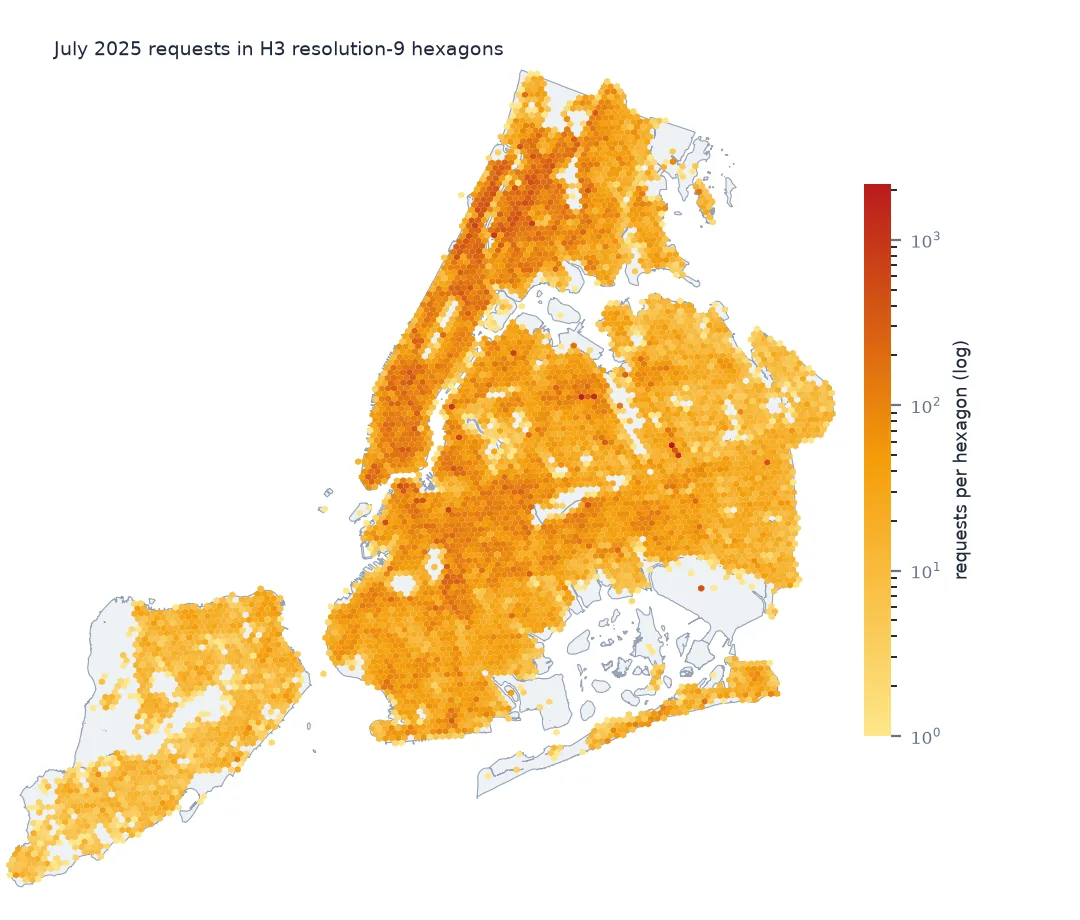
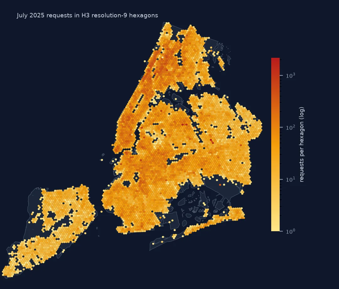
From points to hexagon hotspots

1. Choose the resolution

for r in [7, 8, 9, 10]:
    cc = pd.Series([h3.latlng_to_cell(la, lo, r) for la, lo in zip(pts.latitude.values[:50000], pts.longitude.values[:50000])]).value_counts()
    print(f"res {r}: {h3.average_hexagon_area(r, 'km^2'):.4f} km2, first 50,000 requests fall in {cc.size:,} cells, max {cc.max()}")

res 7: 5.1613 km2, first 50,000 requests fall in 196 cells, max 1510
res 8: 0.7373 km2, first 50,000 requests fall in 1,038 cells, max 504
res 9: 0.1053 km2, first 50,000 requests fall in 5,384 cells, max 474
res 10: 0.0150 km2, first 50,000 requests fall in 16,609 cells, max 352

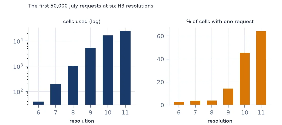
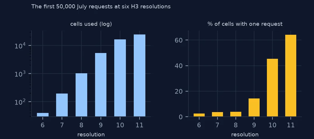
Each finer resolution divides cell area by about seven. At resolution 7 (5.2 km²) the first 50,000 requests fill 196 cells; at 10 (0.015 km²) they spread over 16,609, many with one request. Resolution 9 keeps hotspots a few blocks wide while leaving most cells with enough requests to compare.

2. One address can make a hotspot

top_addr = top.incident_address.value_counts()
print(f"busiest hexagon's requests at its single busiest address: {top_addr.iloc[0] / len(top):.1%} ({top_addr.index[0]})")
addr_share = pts.groupby("hex").incident_address.agg(lambda s: s.value_counts().iloc[0] / len(s) if s.notna().any() else 0)
print(f"hexagons with 200+ requests where one address has more than half: {(addr_share[c[c >= 200].index] > 0.5).mean():.1%}")

busiest hexagon's requests at its single busiest address: 73.2% (78-15 PARSONS BOULEVARD)
hexagons with 200+ requests where one address has more than half: 9.4%

The busiest hexagon is really one address: 73.2% of its requests come from 78-15 Parsons Boulevard. Among hexagons with 200 or more requests, 9.4% have more than half their requests at a single address. A hotspot map of raw requests is partly a map of persistent callers and of specific buildings.

3. Hotspots by complaint type

for t in ["Illegal Parking", "Noise - Residential", "Blocked Driveway", "Noise - Street/Sidewalk"]:
    ct = pts[pts.complaint_type == t].hex.value_counts()
    print(f"{t}: {ct.size:,} hexagons; top 1% hold {ct.head(max(ct.size // 100, 1)).sum() / ct.sum():.1%}")

Illegal Parking: 4,706 hexagons; top 1% hold 18.0%
Noise - Residential: 3,583 hexagons; top 1% hold 14.2%
Blocked Driveway: 3,310 hexagons; top 1% hold 6.0%
Noise - Street/Sidewalk: 2,608 hexagons; top 1% hold 17.8%

Concentration differs by type. The top 1% of hexagons hold 18.0% of illegal-parking requests and 17.8% of street-noise requests, but only 6.0% of blocked-driveway requests, which are spread across residential neighbourhoods with driveways.

4. Smooth with neighbours

smooth = {h: sum(c.get(n, 0) for n in h3.grid_disk(h, 1)) for h in c.index[:2000]}
s = pd.Series(smooth).sort_values(ascending=False)
print(f"top hexagon by own count: {c.index[0]}; by count with its ring of neighbours: {s.index[0]} ({s.iloc[0]:,})")

top hexagon by own count: 892a100eea7ffff; by count with its ring of neighbours: 892a100e8d3ffff (3,781)

Summing each hexagon with its six neighbours (grid_disk with k=1) smooths out single-address spikes: the busiest cell by own count is not the busiest once its ring is included, which reaches 3,781 requests. Smoothing finds areas of concentration rather than individual buildings.

Polygons and parents

The data used on this page

NYC 311 requests created in July 2025 (NYC Open Data, saved copy), indexed with Uber's H3 library.

from pathlib import Path

import geopandas as gpd
import numpy as np
import pandas as pd
import requests

Path("data").mkdir(exist_ok=True)
# NYC 311 Service Requests (NYC Open Data, dataset erm2-nwe9) as queried on 15 October 2026 and saved on this site,
# because requests that are still open keep changing: every request created in July 2025, and the 2025 daily counts by
# agency, complaint type, borough and channel. The queries are in data/README.txt; the live API is
# https://data.cityofnewyork.us/resource/erm2-nwe9.csv
FILES = ["nyc-311-2025-daily-counts-2026-10-15.zip", "nyc-311-2025-07-requests-2026-10-15.zip", "nyc-census-2020-by-geography-2026-10-15.xlsx"]
for name in FILES:
    if not Path(f"data/{name}").exists():
        Path(f"data/{name}").write_bytes(requests.get(f"https://data.spatialworkflow.io/{name}", timeout=600).content)
daily = pd.read_csv("data/nyc-311-2025-daily-counts-2026-10-15.zip", parse_dates=["day"])
july = pd.read_csv("data/nyc-311-2025-07-requests-2026-10-15.zip", low_memory=False,
                   dtype={"unique_key": str, "incident_zip": str, "bbl": str, "community_board": str},
                   parse_dates=["created_date", "closed_date", "resolution_action_updated_date"])
cen = pd.read_excel("data/nyc-census-2020-by-geography-2026-10-15.xlsx", sheet_name="2010, 2020, and Change", skiprows=3)
boro_pop = cen[cen.GeoType == "Boro"].assign(b=lambda d: d.Name.str.upper()).set_index("b").Pop_20
print(f"NYC 311: {daily.n.sum():,} requests in the 2025 daily counts; {len(july):,} requests created in July 2025")

NYC 311: 3,655,042 requests in the 2025 daily counts; 315,883 requests created in July 2025

Example 1: hexagons as polygons

from shapely.geometry import Polygon
hx = gpd.GeoDataFrame({"hex": c.index[:500], "n": c.values[:500]},
                      geometry=[Polygon([(lo, la) for la, lo in h3.cell_to_boundary(h)]) for h in c.index[:500]], crs=4326)
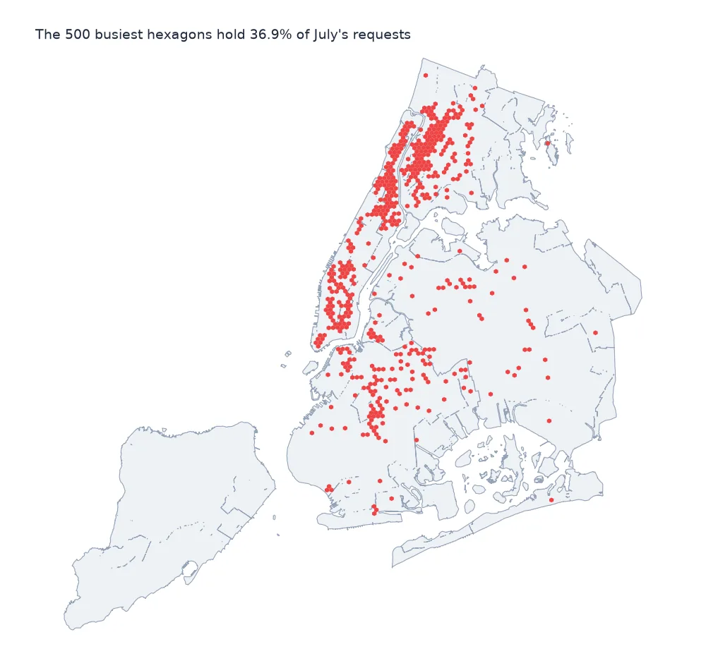
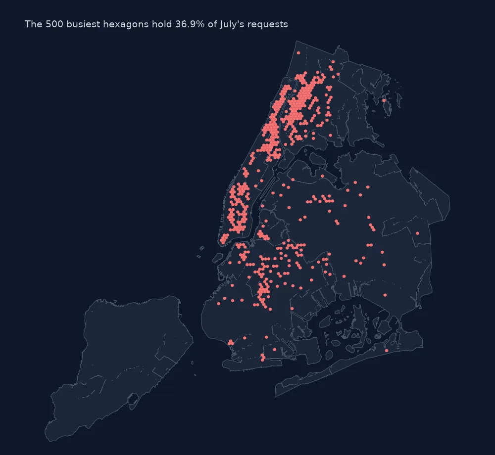
print(f"500 busiest hexagons as polygons: total area {hx.to_crs(32618).area.sum() / 1e6:.1f} km2, holding {hx.n.sum() / c.sum():.1%} of requests")

500 busiest hexagons as polygons: total area 53.0 km2, holding 36.9% of requests

The 500 busiest hexagons cover 53.0 km² — a small part of the city's land — and hold 36.9% of July's requests. Note that cell_to_boundary returns latitude, longitude pairs, which must be swapped for shapely.

Example 2: parent cells

par = pts.hex.map(lambda h: h3.cell_to_parent(h, 7)).value_counts()
print(f"the same requests at resolution 7: {par.size:,} cells; busiest {par.iloc[0]:,}")

the same requests at resolution 7: 203 cells; busiest 10,232

Rolling the same cells up to resolution 7 with cell_to_parent gives 203 cells, the busiest with 10,232 requests: the hierarchy lets you change scale without re-indexing the points.

Why hexagons

Hexagons are the most compact shape that tiles a plane, so every neighbour of a cell is the same distance away and counts are less sensitive to which way a street runs than with squares. H3 adds a global index and a hierarchy, which makes it practical: the cell ID is a column you can group by in pandas or SQL, join across datasets, and aggregate up. H3 explained covers the grid itself.

What hexagons do not fix is what the counts mean. Cells do not have populations, so a hexagon count is a density of requests per area, which favours busy commercial blocks; and a cell with one prolific caller looks like a hotspot. Combine hexagon counts with deduplication and, where it matters, with population or footfall.

Practical notes

• Coordinate order. latlng_to_cell takes latitude first; cell_to_boundary returns (lat, lng) pairs.
• H3 v4 names. Older code uses geo_to_h3 and h3_to_geo_boundary; version 4 renamed them.
• Empty cells have no row; reindex to the cells covering the city if you need zeros.
• Area varies slightly with latitude; within one city it is negligible.

Internal links

• H3 explained — the hexagonal grid
• How to map 311 complaints per resident — neighbourhoods instead of hexagons
• 311 counts inflated by duplicates — why one address can dominate

FAQ

Which H3 resolution should I use for city-level point data?

Resolution 9 (about 0.105 km² per cell) for block-scale hotspots across a city; 8 or 7 for neighbourhood scale.

Why is my busiest H3 cell dominated by one address?

Repeat requests from one building or caller; in July 2025 the busiest cell had 73.2% of its requests at one address.