
How to Read Census Building Permits Survey Data in Python
On this page
Problem statement
The US Census Bureau counts the new homes that local governments authorise every month: each permit-issuing place reports how many buildings they permitted, how many housing units those buildings hold and what they are expected to cost to build. The county files are the easiest way into it, one row per county, every year back to 1990. They are plain comma-separated text, but with two header rows, a blank line, 30-character padded names and two parallel sets of counts, so a plain read_csv gets almost everything wrong. This page reads them properly, with the 2025 file and all 36 annual files, and shows what the rows contain.
Quick answer
Skip the two header rows and the blank line, name the 30 columns yourself, and read the codes as text. The setup below wraps that in permits():
y25 = permits("co2025a.txt")
print(y25[["GEOID", "name", "units", "value"]].sort_values("units", ascending=False).head(5).to_string(index=False))
GEOID name units value
04013 Maricopa County 31651 8516645698
48201 Harris County 30909 7651942703
06037 Los Angeles County 22250 4573893701
48085 Collin County 19082 4745418498
12086 Miami-Dade County 16535 4730017820
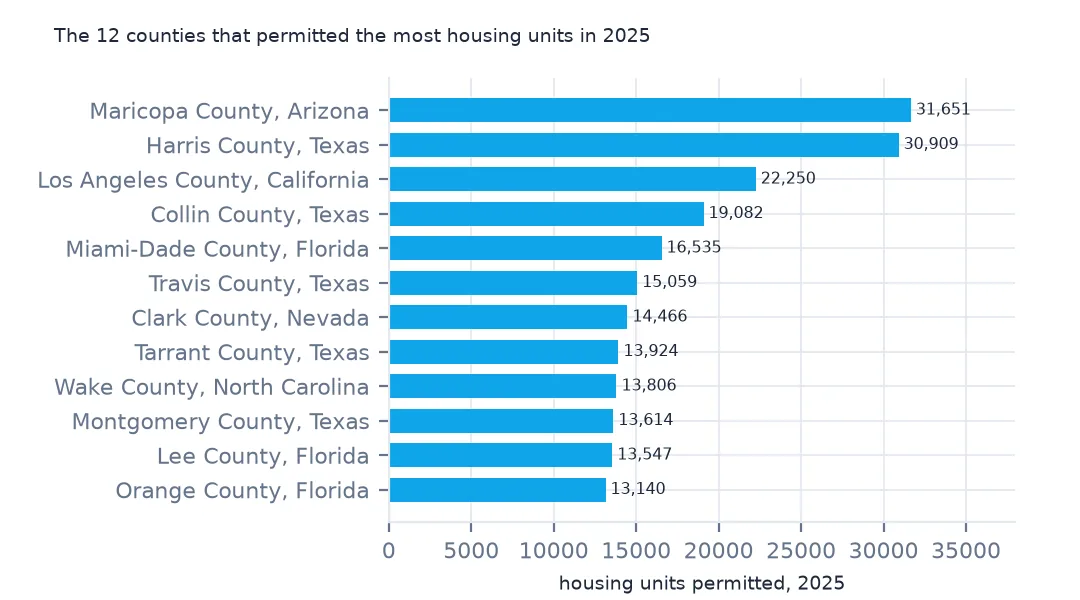
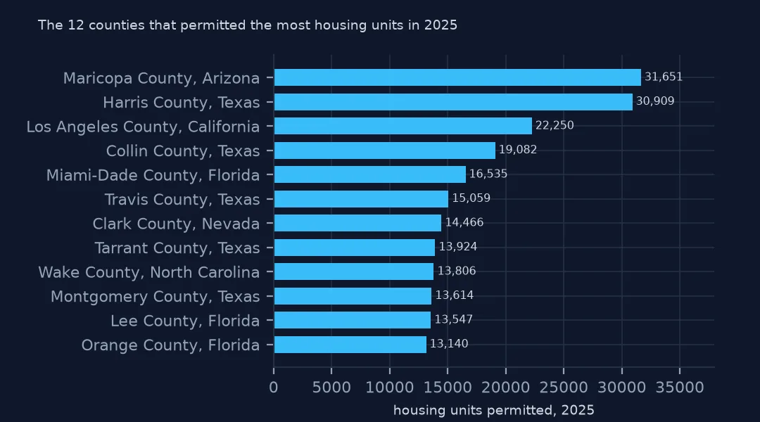
Maricopa County, Arizona, permitted the most housing units in 2025, 31,651, just ahead of Harris County, Texas, with 30,909. value is the declared construction cost in dollars: $8.5 billion in Maricopa.
Header rows, sizes and counties
1. Look at the first lines
for line in Z.open("co2025a.txt").read().decode().splitlines()[:4]:
    print(line[:118])
Survey,FIPS,FIPS,Region,Division,County,,1-unit,,,2-units,,,3-4 units,,,5+ units,,,1-unit rep,,,2-units rep,,,3-4 unit
Date,State,County,Code,Code,Name,Bldgs,Units,Value,Bldgs,Units,Value,Bldgs,Units,Value,Bldgs,Units,Value,Bldgs,Units,V
2025,01,001,3,6,Autauga County ,200,200,82131895,0,0,0,0,0,0,0,0,0,200,200,82131895,0,0,0,0,0,0,0,0,0
The first line names the size of building each group of three columns describes, the second line names the three columns (buildings, units, value), and the third is blank. The rep groups repeat the counts for reported permits only; the first four groups are the Bureau's estimates, which fill in places that did not report. Every county name is padded with spaces to 30 characters.
2. Units by size of building
nat = pd.DataFrame({"buildings": [y25[f"est{s}_bldgs"].sum() for s in SIZES],
                    "units": [y25[f"est{s}_units"].sum() for s in SIZES]},
                   index=["1 unit", "2 units", "3-4 units", "5+ units"])
nat["share of units"] = (nat.units / nat.units.sum()).map("{:.1%}".format)
print(nat.to_string())
buildings units share of units
1 unit 911903 911903 63.7%
2 units 18375 36748 2.6%
3-4 units 5268 18993 1.3%
5+ units 16414 463972 32.4%
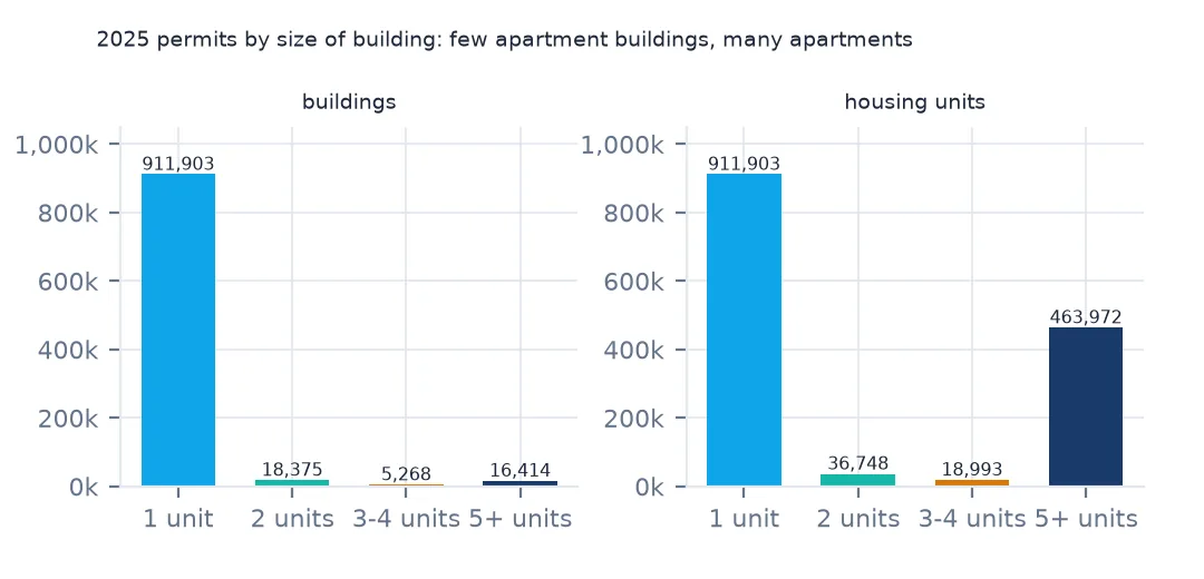
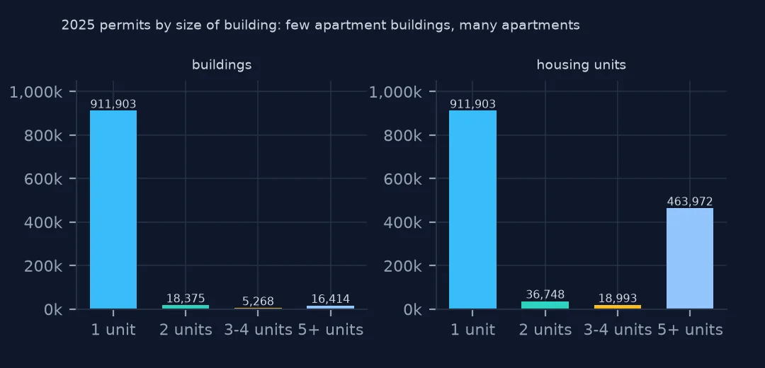
Of the 1,431,616 units permitted in 2025, 63.7% were single-family houses and 32.4% were in buildings of five or more units. The five-plus group is where buildings and units part ways: 16,414 buildings held 463,972 units.
3. Rows that are not counties
odd = y25[~y25.GEOID.isin(pop.GEOID)]
print(odd[["GEOID", "name", "units"]].to_string(index=False))
missing = pop[~pop.GEOID.isin(y25.GEOID)]
print(f"counties with no row: {len(missing)}, population {missing.POPESTIMATE2025.sum():,}; rows with zero units: {(y25.units == 0).sum()}")
GEOID name units
23000 Maine Unorganized Territory 114
26000 Michigan Balance of State 135
30000 Montana Balance of State 0
35000 New Mexico Balance of State 2752
41000 Oregon Balance of State 169
counties with no row: 120, population 797,240; rows with zero units: 248
Five rows have county code 000. They are permits from places the Census Bureau does not assign to a single county: Maine's unorganized territory and "Balance of State" rows for Michigan, Montana, New Mexico and Oregon. New Mexico's holds 2,752 units, enough to matter in a state total but impossible to map. In the other direction, 120 counties, home to 797,240 people, have no row at all, because no place in them issues permits, and 248 rows are present with zero units. A missing county is unknown, not zero.
States, years and a county map
The data used on this page
The US Census Bureau's Building Permits Survey county files (annual 1990–2025 and year-to-date 2025–2026), its Northeast place files for 2020–2025, the Vintage 2025 county population estimates and the 2024 cartographic boundary counties, all public domain. They were downloaded on 16 October 2026 and saved on this site in one archive, because Census revises recent months as late reports arrive.
from pathlib import Path
import zipfile

import geopandas as gpd
import numpy as np
import pandas as pd
import requests

Path("data").mkdir(exist_ok=True)
# US Census Bureau Building Permits Survey: annual county files co1990a.txt-co2025a.txt, year-to-date county files
# co2501y.txt-co2512y.txt and co2601y.txt-co2608y.txt, Northeast place files ne2020a.txt-ne2025a.txt; the Vintage 2025
# county population estimates; 2024 cartographic boundary counties. Downloaded 16 October 2026, saved here unchanged.
# Live: https://www2.census.gov/econ/bps/County/co2025a.txt (and the same folder for the others),
# https://www2.census.gov/econ/bps/Place/Northeast%20Region/ne2025a.txt,
# https://www2.census.gov/programs-surveys/popest/datasets/2020-2025/counties/totals/co-est2025-alldata.csv,
# https://www2.census.gov/geo/tiger/GENZ2024/shp/cb_2024_us_county_20m.zip
ARCHIVE = "census-building-permits-2026-10-16.zip"
if not Path(f"data/{ARCHIVE}").exists():
    Path(f"data/{ARCHIVE}").write_bytes(requests.get(f"https://data.spatialworkflow.io/{ARCHIVE}", timeout=600).content)
Z = zipfile.ZipFile(f"data/{ARCHIVE}")

SIZES = ["1", "2", "34", "5"]  # buildings with 1 unit, 2 units, 3-4 units, 5 or more units
COLS = (["survey", "state", "county", "region", "division", "name"]
        + [f"{k}{s}_{m}" for k in ("est", "rep") for s in SIZES for m in ("bldgs", "units", "value")])


def permits(name):
    """One county file: two header rows and a blank line, then a row per county. est = estimate with
    imputation for places that did not report, rep = reported only."""
    d = pd.read_csv(Z.open(name), skiprows=3, header=None, names=COLS, skipinitialspace=True,
                    dtype={"survey": str, "state": str, "county": str, "name": str})
    d["survey"], d["name"] = d.survey.str.strip(), d.name.str.strip()
    d["state"], d["county"] = d.state.str.strip().str.zfill(2), d.county.str.strip().str.zfill(3)
    return d.assign(GEOID=d.state + d.county,
                    units=d[[f"est{s}_units" for s in SIZES]].sum(axis=1),
                    reported=d[[f"rep{s}_units" for s in SIZES]].sum(axis=1),
                    value=d[[f"est{s}_value" for s in SIZES]].sum(axis=1))


pop = pd.read_csv(Z.open("co-est2025-alldata.csv"), encoding="latin-1", dtype={"STATE": str, "COUNTY": str})
pop = pop[pop.SUMLEV == 50].assign(GEOID=lambda p: p.STATE + p.COUNTY)
Path("data/cb_2024_us_county_20m.zip").write_bytes(Z.read("cb_2024_us_county_20m.zip"))
counties = gpd.read_file("data/cb_2024_us_county_20m.zip")
counties = counties[~counties.STUSPS.isin(["AK", "HI", "PR"])].to_crs(5070)
y25 = permits("co2025a.txt")
print(f"2025 county file: {len(y25):,} rows, {y25.units.sum():,} units permitted; {len(pop):,} counties in the estimates")
2025 county file: 3,029 rows, 1,431,616 units permitted; 3,144 counties in the estimates
Example 1: units by state
st = y25.merge(pop[["GEOID", "STNAME"]], on="GEOID").groupby("STNAME").units.sum().sort_values(ascending=False)
print(st.head(6).to_string())
print(f"top 3 states: {st.head(3).sum() / y25.units.sum():.1%} of all units")
STNAME
Texas 210217
Florida 178297
California 103856
North Carolina 86167
Georgia 61196
Arizona 51532
top 3 states: 34.4% of all units
Texas, Florida and California permitted 34.4% of all units in 2025; Texas alone 210,217. The state comes from the first two digits of GEOID, so the names here come from the population estimates, which spell every state out.
Example 2: all 36 annual files in one frame
years = pd.concat([permits(f"co{y}a.txt").assign(year=y) for y in range(1990, 2026)], ignore_index=True)
by_year = years.groupby("year").agg(rows=("GEOID", "size"), units=("units", "sum"))
print(by_year.loc[[1990, 2005, 2009, 2025]].to_string())
print(f"survey codes: {years.groupby('year').survey.first().loc[[1990, 1998, 1999]].tolist()}")
rows units
year
1990 2994 1118551
2005 3027 2155316
2009 3026 582963
2025 3029 1431616
survey codes: ['9099', '9899', '1999']
The 36 files stack into one frame with a year column. The national total runs from 2,155,316 units in 2005, the peak of the housing boom, to 582,963 in 2009. Before 1999 the survey date is written as 9099, 9199 and so on through 9899, so take the year from the file name, not from that column.
Example 3: a county map
m = counties.merge(y25[["GEOID", "units"]], on="GEOID", how="left")
print(f"counties drawn: {len(m):,}; with a permit row: {m.units.notna().sum():,}; 1,000+ units: {(m.units >= 1000).sum()}")
ax = m.plot(column=np.log10(m.units.fillna(0) + 1), cmap="YlOrRd", missing_kwds={"color": "lightgrey"}, figsize=(10, 6))
ax.set_axis_off()
counties drawn: 3,109; with a permit row: 2,995; 1,000+ units: 329
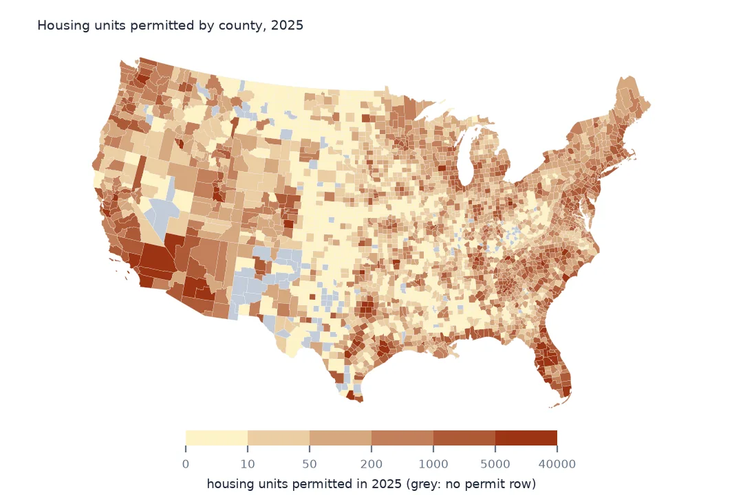
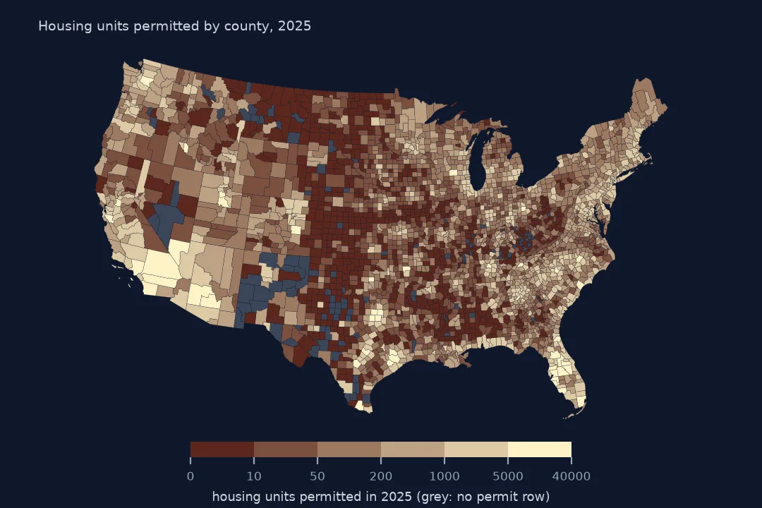
Of the 3,109 counties drawn in the lower 48, 2,995 have a permit row and 329 permitted 1,000 or more units. The grey counties are the ones with no permit-issuing place.
Internal links
- Housing permits per 1,000 residents — the map scaled by population
- US housing permits since 1990 — the 36 files as a time series
- Units, buildings and value — what each column counts
- Reported against imputed units — the two sets of columns
- Census permit files with two header rows — what a plain
read_csvdoes to them
FAQ
Where do I download US building permit data by county?
From the Census Bureau's BPS county folder: coYYYYa.txt is the annual file for year YYYY, coYYMMy.txt the year to date to month MM. They are comma-separated text with two header rows.