
How to Map New Housing Permits per 1,000 Residents by County
On this page
Problem statement
A map of housing permits by county is mostly a map of population: Maricopa and Harris counties permit the most because they are the biggest. To see where building is fast for the size of the place, divide by residents. That needs the Census Bureau's permit file joined to its population estimates on the five-digit county code, a decision about counties with no permit row, and some care with small counties, where one subdivision is a large share. This page maps 2025 permits per 1,000 residents, ranks counties and states, and compares one year with a five-year average.
Quick answer
Join the permit file to the Vintage 2025 population estimates on GEOID, keeping every county in the estimates, and divide:
rate = pop[["GEOID", "STNAME", "CTYNAME", "POPESTIMATE2025"]].merge(y25[["GEOID", "units"]], on="GEOID", how="left")
rate["per_1000"] = rate.units / rate.POPESTIMATE2025 * 1000
print(f"US: {rate.units.sum() / rate.POPESTIMATE2025.sum() * 1000:.2f} units per 1,000 residents; county median {rate.per_1000.median():.2f}")
US: 4.18 units per 1,000 residents; county median 2.08
The US permitted 4.18 units per 1,000 residents in 2025, but the median county only 2.08: the counties that build most are also the larger ones.
Joining permits to population
1. Join on the five-digit code, keep the gaps
print(f"counties: {len(rate):,}; no permit row: {rate.units.isna().sum()}; zero units: {(rate.units == 0).sum()}")
print(rate[rate.units.isna()].nlargest(3, "POPESTIMATE2025")[["STNAME", "CTYNAME", "POPESTIMATE2025"]].to_string(index=False))
counties: 3,144; no permit row: 120; zero units: 247
STNAME CTYNAME POPESTIMATE2025
Nevada Nye County 57336
New Mexico Rio Arriba County 39832
Indiana Greene County 31165
A left join from the estimates keeps all 3,144 counties. 120 have no permit row, among them Nye County, Nevada, with 57,336 residents, and 247 have a row with zero units. Leave the 120 as missing on the map rather than filling them with zero: no place there issues permits, so the survey simply does not see what is built.
2. The highest rates
big = rate[rate.POPESTIMATE2025 >= 50_000]
print(f"counties of 50,000+ residents: {len(big):,}")
print(big.nlargest(8, "per_1000")[["CTYNAME", "STNAME", "POPESTIMATE2025", "units", "per_1000"]].round(1).to_string(index=False))
counties of 50,000+ residents: 1,014
CTYNAME STNAME POPESTIMATE2025 units per_1000
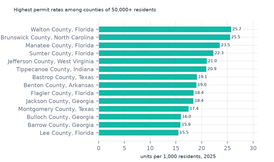
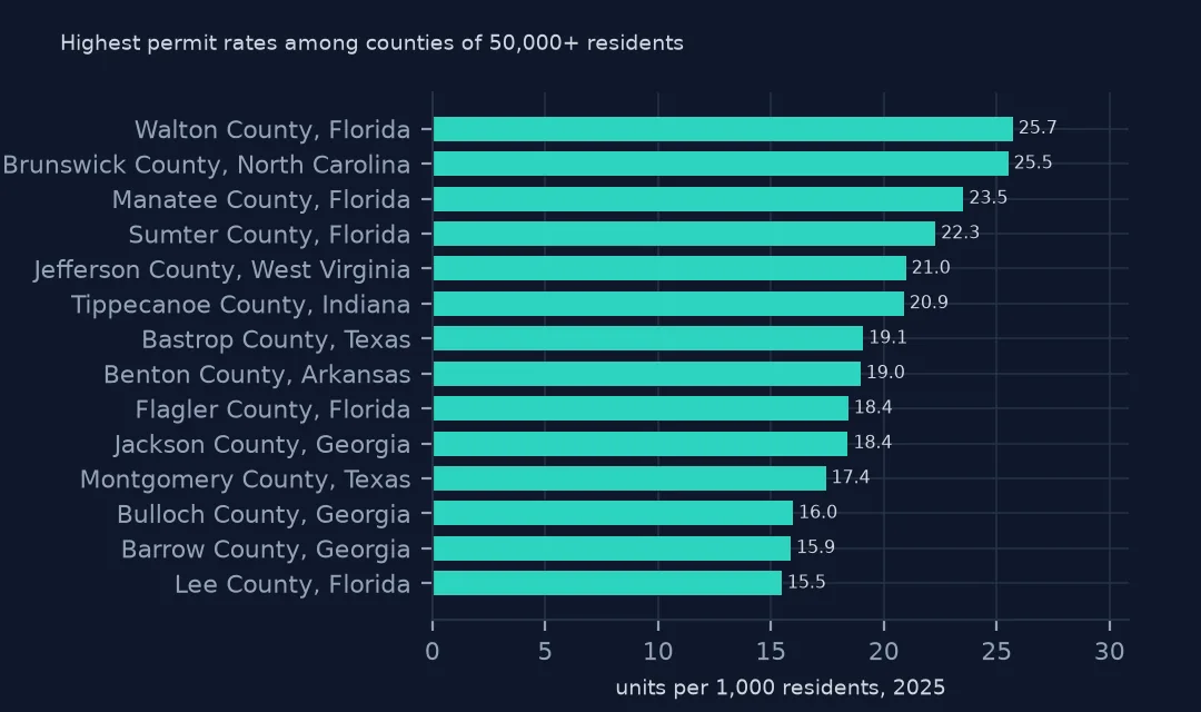
Walton County Florida 93288 2399.0 25.7
Brunswick County North Carolina 174702 4457.0 25.5
Manatee County Florida 468200 11015.0 23.5
Sumter County Florida 157772 3516.0 22.3
Jefferson County West Virginia 63102 1324.0 21.0
Tippecanoe County Indiana 190456 3979.0 20.9
Bastrop County Texas 118908 2269.0 19.1
Benton County Arkansas 332554 6307.0 19.0
Among counties of 50,000 or more, Walton County on Florida's Panhandle permitted 25.7 units per 1,000 residents, ahead of Brunswick County, North Carolina, at 25.5. Florida has three of the top four. Sumter County, home of The Villages, is fourth at 22.3, but none of its 3,516 units were reported: the whole figure is the Bureau's estimate (see the imputation page).
3. Small counties swing
rate["size"] = pd.cut(rate.POPESTIMATE2025, [0, 10_000, 50_000, 250_000, 1e8], labels=["under 10,000", "10,000-50,000", "50,000-250,000", "250,000+"])
print(rate.groupby("size", observed=True).per_1000.describe()[["count", "50%", "std", "max"]].round(2).to_string())
count 50% std max
size
under 10,000 641.0 0.83 3.55 30.99
10,000-50,000 1370.0 1.78 3.46 48.22
50,000-250,000 719.0 3.23 3.65 25.72
250,000+ 294.0 3.46 3.79 23.53
The median rate climbs with county size, from 0.83 per 1,000 in counties under 10,000 people to 3.46 in counties of 250,000 or more, while the spread is about the same in every class (a standard deviation near 3.5). The single highest rate, 48.22, belongs to a county of 10,000 to 50,000, where a few hundred homes are a large share.
States, five years and the map
The data used on this page
The US Census Bureau's Building Permits Survey county files (annual 1990–2025 and year-to-date 2025–2026), its Northeast place files for 2020–2025, the Vintage 2025 county population estimates and the 2024 cartographic boundary counties, all public domain. They were downloaded on 16 October 2026 and saved on this site in one archive, because Census revises recent months as late reports arrive.
from pathlib import Path
import zipfile

import geopandas as gpd
import numpy as np
import pandas as pd
import requests

Path("data").mkdir(exist_ok=True)
# US Census Bureau Building Permits Survey: annual county files co1990a.txt-co2025a.txt, year-to-date county files
# co2501y.txt-co2512y.txt and co2601y.txt-co2608y.txt, Northeast place files ne2020a.txt-ne2025a.txt; the Vintage 2025
# county population estimates; 2024 cartographic boundary counties. Downloaded 16 October 2026, saved here unchanged.
# Live: https://www2.census.gov/econ/bps/County/co2025a.txt (and the same folder for the others),
# https://www2.census.gov/econ/bps/Place/Northeast%20Region/ne2025a.txt,
# https://www2.census.gov/programs-surveys/popest/datasets/2020-2025/counties/totals/co-est2025-alldata.csv,
# https://www2.census.gov/geo/tiger/GENZ2024/shp/cb_2024_us_county_20m.zip
ARCHIVE = "census-building-permits-2026-10-16.zip"
if not Path(f"data/{ARCHIVE}").exists():
    Path(f"data/{ARCHIVE}").write_bytes(requests.get(f"https://data.spatialworkflow.io/{ARCHIVE}", timeout=600).content)
Z = zipfile.ZipFile(f"data/{ARCHIVE}")

SIZES = ["1", "2", "34", "5"]  # buildings with 1 unit, 2 units, 3-4 units, 5 or more units
COLS = (["survey", "state", "county", "region", "division", "name"]
        + [f"{k}{s}_{m}" for k in ("est", "rep") for s in SIZES for m in ("bldgs", "units", "value")])


def permits(name):
    """One county file: two header rows and a blank line, then a row per county. est = estimate with
    imputation for places that did not report, rep = reported only."""
    d = pd.read_csv(Z.open(name), skiprows=3, header=None, names=COLS, skipinitialspace=True,
                    dtype={"survey": str, "state": str, "county": str, "name": str})
    d["survey"], d["name"] = d.survey.str.strip(), d.name.str.strip()
    d["state"], d["county"] = d.state.str.strip().str.zfill(2), d.county.str.strip().str.zfill(3)
    return d.assign(GEOID=d.state + d.county,
                    units=d[[f"est{s}_units" for s in SIZES]].sum(axis=1),
                    reported=d[[f"rep{s}_units" for s in SIZES]].sum(axis=1),
                    value=d[[f"est{s}_value" for s in SIZES]].sum(axis=1))


pop = pd.read_csv(Z.open("co-est2025-alldata.csv"), encoding="latin-1", dtype={"STATE": str, "COUNTY": str})
pop = pop[pop.SUMLEV == 50].assign(GEOID=lambda p: p.STATE + p.COUNTY)
Path("data/cb_2024_us_county_20m.zip").write_bytes(Z.read("cb_2024_us_county_20m.zip"))
counties = gpd.read_file("data/cb_2024_us_county_20m.zip")
counties = counties[~counties.STUSPS.isin(["AK", "HI", "PR"])].to_crs(5070)
y25 = permits("co2025a.txt")
print(f"2025 county file: {len(y25):,} rows, {y25.units.sum():,} units permitted; {len(pop):,} counties in the estimates")
2025 county file: 3,029 rows, 1,431,616 units permitted; 3,144 counties in the estimates
Example 1: by state
s = rate.groupby("STNAME")[["units", "POPESTIMATE2025"]].sum()
s["per_1000"] = s.units / s.POPESTIMATE2025 * 1000
s = s.sort_values("per_1000")
print("lowest:", ", ".join(f"{k} {v:.2f}" for k, v in s.per_1000.head(4).items()))
print("highest:", ", ".join(f"{k} {v:.2f}" for k, v in s.per_1000.tail(4).items()))
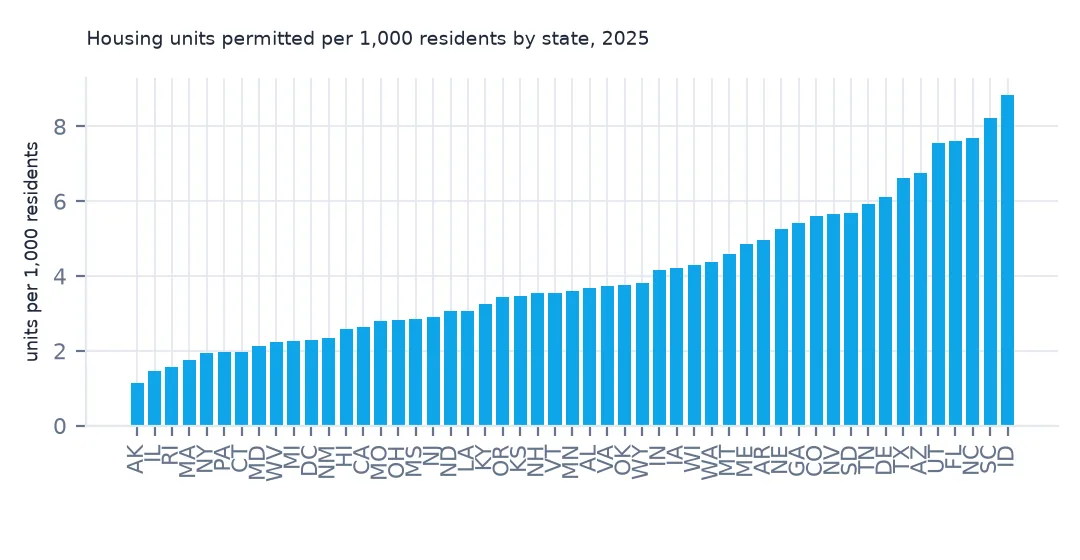
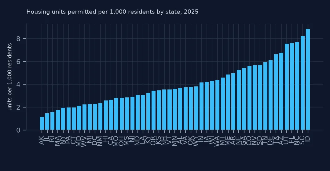
lowest: Alaska 1.15, Illinois 1.46, Rhode Island 1.56, Massachusetts 1.74
highest: Florida 7.60, North Carolina 7.69, South Carolina 8.23, Idaho 8.84
Idaho permitted the most per resident, 8.84 per 1,000, followed by South Carolina, North Carolina and Florida. Alaska, Illinois, Rhode Island and Massachusetts permitted the least, under 1.8.
Example 2: five years instead of one
five = pd.concat([permits(f"co{y}a.txt") for y in range(2021, 2026)]).groupby("GEOID").units.sum().rename("units_5y")
r5 = rate.merge(five, on="GEOID", how="left")
r5["per_1000_yr"] = r5.units_5y / 5 / r5.POPESTIMATE2025 * 1000
small = r5[r5.POPESTIMATE2025 < 10_000]
print(f"counties under 10,000 people: one-year rate std {small.per_1000.std():.2f}, five-year average std {small.per_1000_yr.std():.2f}")
print(f"rank correlation of 2025 with the five-year average: {r5.per_1000.corr(r5.per_1000_yr, method='spearman'):.2f}")
counties under 10,000 people: one-year rate std 3.55, five-year average std 3.45
rank correlation of 2025 with the five-year average: 0.93
Averaging 2021–2025 barely calms the small counties: their standard deviation falls only from 3.55 to 3.45, and the 2025 ranking correlates at 0.93 with the five-year one. The high small-county rates are steady growth, not a one-year spike. Connecticut needs care here: its 2021 and 2022 rows use the old county codes, so only three of its five years join to the 2025 estimates.
Example 3: the map
m = counties.merge(r5[["GEOID", "per_1000_yr"]], on="GEOID", how="left")
bins = [0, 1, 2, 4, 6, 10, 15, 1000]
m["cls"] = pd.cut(m.per_1000_yr, bins, right=False)
print(m.cls.value_counts(sort=False).to_string())
ax = m.plot(column="cls", cmap="YlGnBu", legend=True, missing_kwds={"color": "lightgrey"}, figsize=(10, 6))
ax.set_axis_off()
cls
[0, 1) 876
[1, 2) 547
[2, 4) 758
[4, 6) 337
[6, 10) 339
[10, 15) 103
[15, 1000) 46
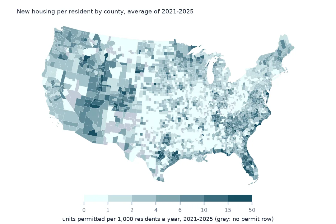
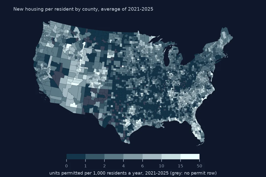
46 counties averaged 15 or more units per 1,000 residents a year, and 876 under one. Fast building runs along the South Atlantic coast, through central Texas and the Mountain West; the slow counties fill the Great Plains, Appalachia and the industrial Midwest.
Internal links
- Read the permit files — the files and the
permits()reader - Permits against population growth — whether building keeps up with arrivals
- The apartment share of new housing — what kind of housing the rate counts
- Connecticut's planning regions — why its 2021 rows will not join
FAQ
Which US county permits the most housing per person?
Among counties of 50,000 or more, Walton County, Florida, with 25.7 units per 1,000 residents in 2025, then Brunswick County, North Carolina (25.5) and Manatee County, Florida (23.5).