
Vegetation indices explained: NDVI, EVI, NDRE and when each fails
Problem statement
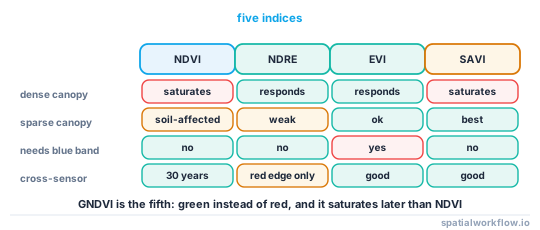
NDVI is the default and it stops working exactly where agriculture gets interesting. Once a canopy closes, almost all the red light is absorbed, the numerator and denominator both flatten, and the index becomes nearly constant across a wide range of real biomass.
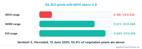
That is not a theoretical concern. On a cloud-free Sentinel-2 scene over Dutch arable land in mid-June, 64,302 vegetation pixels had an NDVI above 0.8. Across those pixels NDVI varied over a range of 0.128 with a coefficient of variation of 0.032; the red-edge index NDRE over the same pixels varied over a range of 0.572 with a coefficient of variation of 0.098 — three times the relative variation, on the same ground.
This guide covers the main indices, what each responds to, and where each stops responding.
Quick answer
import numpy as np

ndvi  = (nir - red) / (nir + red)
ndre  = (nir - rededge1) / (nir + rededge1)          # Sentinel-2 B8 and B5
evi   = 2.5 * (nir - red) / (nir + 6 * red - 7.5 * blue + 1)
evi2  = 2.5 * (nir - red) / (nir + 2.4 * red + 1)     # no blue band needed
gndvi = (nir - green) / (nir + green)
savi  = 1.5 * (nir - red) / (nir + red + 0.5)         # soil-adjusted, sparse canopies
Reflectance must be scaled first: Sentinel-2 L2A stores reflectance × 10,000, so divide by 10,000 before any index. Skipping that makes EVI, EVI2 and SAVI wrong, because their additive constants assume reflectance in 0–1.
Step-by-step solution
1. Know what NDVI actually measures
The contrast between red absorption by chlorophyll and near-infrared scattering by leaf structure. That contrast grows quickly as leaf area increases from bare soil and then flattens, because there is no more red light left to absorb. The index saturates; the canopy does not.
2. Use a red-edge index where the canopy is closed
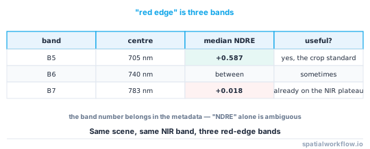
The red edge — Sentinel-2 bands 5, 6 and 7 between about 705 and 783 nm — sits on the steep part of the vegetation reflectance curve, so it keeps responding when red is exhausted. Measured on 101 fields whose median NDVI exceeded 0.8, NDVI spanned 0.102 across the fields and NDRE spanned 0.264.
3. Choose the right red-edge band
Not all of them work. Using band 7 at 783 nm gives an index near zero, because that band is already on the NIR plateau: the same scene gave a median NDRE of +0.587 with band 5 and +0.018 with band 7. Band 5 is the usual choice for crop work.
4. Use a soil-adjusted index on sparse canopies
At low cover, NDVI is strongly affected by the soil beneath — wet soil and dry soil give different values under identical vegetation. SAVI adds a soil brightness term; it matters in early season, in arid systems and on row crops before closure.
5. Use EVI where the atmosphere or the background is a problem
EVI adds a blue-band aerosol correction and a canopy background adjustment. It is more responsive at high biomass than NDVI — on the dense pixels above it varied over 0.684 against NDVI's 0.128 — at the cost of needing a blue band whose atmospheric correction is the least reliable of the three.
6. Match the index to the question, not to the convention
Cover and greenness: NDVI. Biomass or nitrogen at closure: NDRE. Early-season emergence on bare soil: SAVI. Cross-sensor consistency over decades: NDVI, because it is the one everybody else used.
7. Mask before you index
Cloud, shadow, water and cloud shadow all produce valid-looking index values. Sentinel-2's scene classification layer at 20 m is the cheapest mask available; on the reference scene, classes 4, 5 and 6 — vegetation, bare soil and water — covered the usable ground and class 4 alone was 81.2%.
Code examples
Example 1 — compute the family, correctly scaled and masked
import numpy as np, rasterio

SCALE = 1e-4                      # Sentinel-2 L2A reflectance is stored as x10,000

def indices(red, nir, rededge1, blue, green, scl=None):
    red, nir, re1, blue, green = (a.astype("float32") * SCALE
                                  for a in (red, nir, rededge1, blue, green))
    with np.errstate(invalid="ignore", divide="ignore"):
        out = {
            "ndvi": (nir - red) / (nir + red),
            "ndre": (nir - re1) / (nir + re1),
            "gndvi": (nir - green) / (nir + green),
            "evi": 2.5 * (nir - red) / (nir + 6 * red - 7.5 * blue + 1),
            "evi2": 2.5 * (nir - red) / (nir + 2.4 * red + 1),
            "savi": 1.5 * (nir - red) / (nir + red + 0.5),
        }
    if scl is not None:
        keep = np.isin(scl, [4, 5, 6])           # vegetation, bare soil, water
        for k in out:
            out[k] = np.where(keep, out[k], np.nan)
    return out
Example 2 — measure the saturation on your own scene
import numpy as np

veg = np.isin(scl, [4]) & np.isfinite(ndvi) & np.isfinite(ndre)
dense = veg & (ndvi > 0.8)
print(f"vegetation pixels {veg.sum():,}; dense canopy {dense.sum():,} "
      f"({dense.sum()/veg.sum():.1%})")

for name, arr in (("NDVI", ndvi), ("NDRE", ndre), ("EVI", evi)):
    v = arr[dense]
    print(f"{name:5} range {v.max()-v.min():.3f}  sd {v.std():.4f}  "
          f"CV {v.std()/abs(v.mean()):.3f}")
vegetation pixels 114,973; dense canopy 64,302 (55.9%)
NDVI range 0.128 sd 0.0278 CV 0.032
NDRE range 0.572 sd 0.0644 CV 0.098
EVI range 0.684 sd 0.0807 CV 0.106
Run this on your own peak-season scene before choosing an index. If more than half your vegetation pixels are above 0.8, NDVI is not going to separate them.
Example 3 — choosing the red-edge band matters
import numpy as np

ndre_b5 = (nir - b5) / (nir + b5)          # 705 nm — on the red edge
ndre_b7 = (nir - b7) / (nir + b7)          # 783 nm — already on the NIR plateau

for name, arr in (("NDRE B5", ndre_b5), ("NDRE B7", ndre_b7)):
    v = arr[veg]
    print(f"{name}: p5 {np.percentile(v,5):+.3f}  median {np.median(v):+.3f}  "
          f"p95 {np.percentile(v,95):+.3f}")
NDRE B5: p5 +0.319 median +0.587 p95 +0.749
NDRE B7: p5 -0.070 median +0.018 p95 +0.096
Band 7 is close enough to the NIR plateau that the normalised difference collapses towards zero. "Red edge" is three bands with quite different behaviour, and the band number belongs in the metadata.
Explanation
Why NDVI saturates and a red-edge index does not
Chlorophyll absorbs red light strongly. Once the leaf area index passes about three, essentially all incident red is absorbed, so further leaves change red reflectance almost not at all while NIR keeps rising slowly. The normalised difference therefore asymptotes. The red edge sits where absorption is only partial, so additional chlorophyll still changes the reflectance measurably — which is why red-edge indices track nitrogen status and late-season biomass where NDVI is flat.
Why the additive constants mean reflectance must be scaled
EVI's +1, EVI2's +1 and SAVI's +0.5 are in reflectance units. Feeding raw digital numbers in the thousands makes those constants negligible, and the index silently becomes a different formula — usually close to a scaled NDVI. NDVI and NDRE are ratios and survive an unscaled input; the others do not.
Why SAVI exists
At low cover the soil contributes most of the signal, and soil brightness varies with moisture, tillage and organic matter. NDVI over 20% cover on wet dark soil and on dry bright soil differs measurably with identical vegetation. SAVI's L term compresses that, at the cost of a constant that is itself cover-dependent — which is why adaptive variants exist.
Why NDVI remains the right answer surprisingly often
Three decades of consistent measurement across AVHRR, MODIS, Landsat and Sentinel means NDVI has a comparability nothing else has. For trend work, for cross-sensor time series and for anything that has to line up with published literature, the saturation is a known limitation rather than a reason to switch.
Edge cases or notes
- Scale reflectance first. EVI, EVI2 and SAVI depend on it; NDVI and NDRE do not.
- Band resolutions differ. Red and NIR are 10 m on Sentinel-2; the red edges are 20 m.
- L2A includes an aerosol correction that the blue band, and so EVI, depends on most.
- Negative NDVI is water, not an error.
- Shadow looks like dense canopy to most indices; mask it.
- Different sensors have different band centres, so indices are not directly comparable.
- Sun and view angle matter more at high biomass than most people assume.
- Record which bands you used. "NDRE" without a band number is ambiguous.
Internal links
- NDVI stops responding in a dense canopy — what to do about it
- Crop phenology and growing seasons explained — the seasonal curve these indices trace
- How to extract phenology metrics from an NDVI time series — using the curve
- Spectral indices explained — the wider family
- How to calculate NDVI in Python — the basic computation
- How to mask clouds in Sentinel-2 imagery in Python — the SCL mask
- NDVI values are out of range — scaling and nodata problems
- How to classify crop types from a satellite time series — where band choice decides the result
FAQ
Why does my NDVI stop changing in summer?
Because the canopy has closed and almost all red light is already absorbed. On a real June scene, 55.9% of vegetation pixels were above 0.8 and varied over a range of only 0.128.
What should I use instead of NDVI at high biomass?
A red-edge index such as NDRE, or EVI. On the same dense pixels, NDRE varied over 0.572 and EVI over 0.684.
Which red-edge band should I use?
Sentinel-2 band 5 at 705 nm for crops. Band 7 at 783 nm is already on the NIR plateau and gives an index near zero.
Do I need to scale reflectance before computing indices?
For EVI, EVI2 and SAVI, yes — their additive constants are in reflectance units. NDVI and NDRE are ratios and are unaffected.
When is SAVI worth using?
On sparse canopies, where soil brightness dominates the signal — early season, arid systems and row crops before closure.
Is NDVI obsolete?
No. Its cross-sensor consistency over three decades is unmatched, which is exactly what trend work and comparison with published literature need.