
How to Read UK Road Traffic Counts in Python
On this page
Problem statement
The Department for Transport publishes a traffic figure for every road it counts in Great Britain: the annual average daily flow (AADF), split by vehicle type, for 46,754 count points between 2000 and 2025. It is the most detailed open picture of where traffic goes in any country, and one CSV of 600,551 rows. Reading it is straightforward; reading it correctly needs four things the file does not shout about: most of its values are estimates rather than counts, major roads are links with a length while minor roads are points without one, the road categories are codes, and the vehicle classes are rounded separately.
This page loads the file, walks through what a row is and what each group of columns means, and checks the parts that later analyses depend on.
Quick answer
Read the CSV, take one year, and summarise by road category — which also shows how many of the values were actually counted that year:
y = aadf[aadf.year == 2025]
print(y.groupby("road_category").agg(points=("count_point_id", "size"), median_aadf=("all_motor_vehicles", "median"),
                                     counted=("estimation_method", lambda s: (s == "Counted").mean())).round(2).to_string())
points median_aadf counted
road_category
MB 542 5234.0 0.84
MCU 3851 1047.0 0.85
PA 14453 13306.0 0.17
PM 35 62118.0 0.34
TA 2214 22244.5 0.48
TM 1239 72424.0 0.61
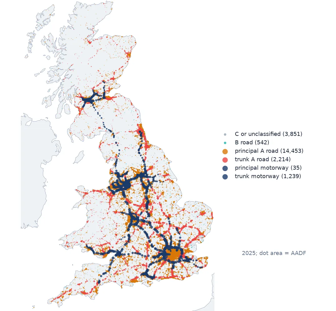
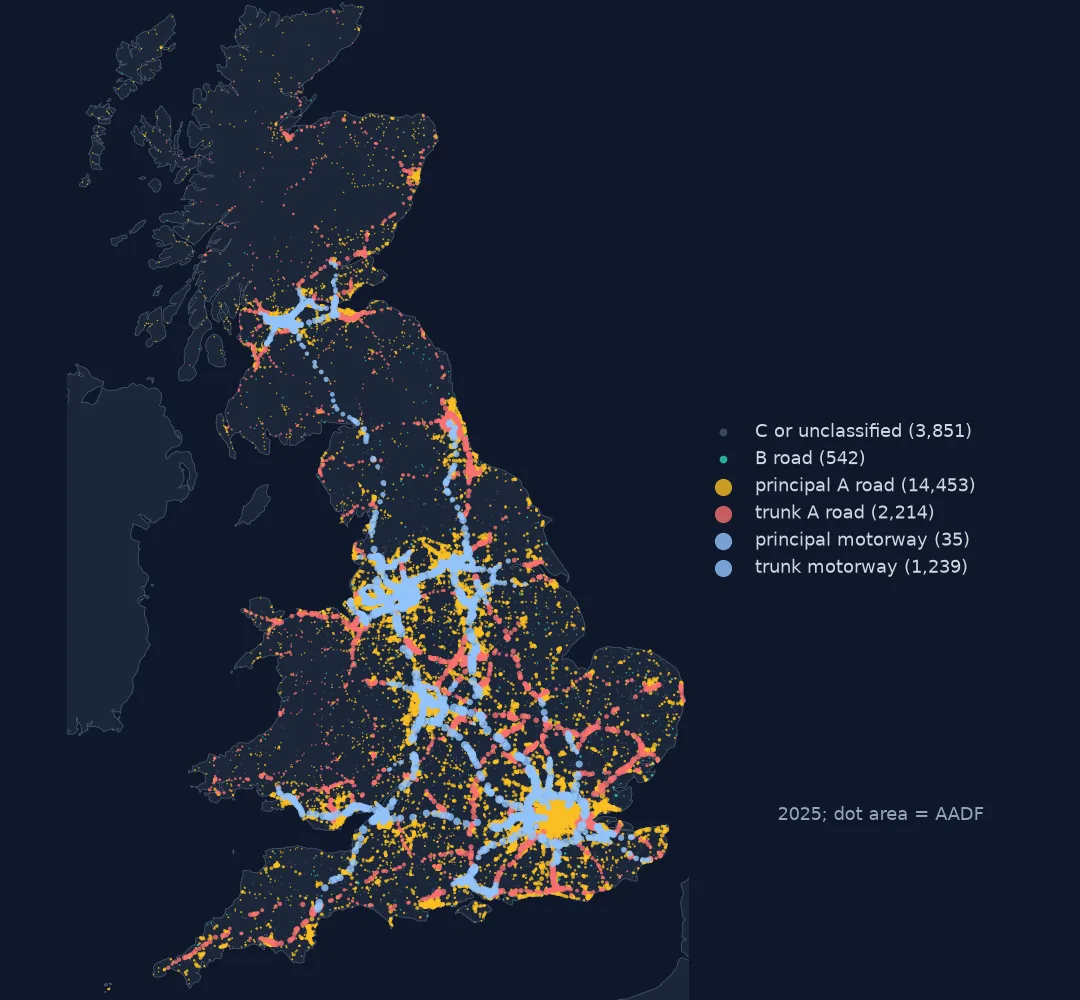
In 2025 the file has 14,453 count points on principal A roads (PA), 2,214 on trunk A roads (TA), 1,239 on trunk motorways (TM) and 35 on principal motorways (PM), plus 542 on B roads (MB) and 3,851 on C and unclassified roads (MCU). A median motorway point carries 72,424 vehicles a day, a C road 1,047. Only 17% of the principal A-road values in 2025 were counted; on minor roads 84–85% were.
What a row is
1. One row per count point per year
print(aadf.duplicated(["count_point_id", "year"]).sum(), "duplicate point-years")
cp = aadf[aadf.count_point_id == aadf.count_point_id.iloc[0]]
print(cp[["year", "road_name", "estimation_method_detailed", "all_motor_vehicles"]].head(6).to_string(index=False))
years = aadf.groupby("count_point_id").year.agg(["min", "max", "size"])
print(f"years per count point: median {years['size'].median():.0f}; points present in every year 2000-2025: {(years['size'] == 26).sum():,}")
0 duplicate point-years
year road_name estimation_method_detailed all_motor_vehicles
2000 A3111 Estimated using AADF from previous year on this link 1430
2001 A3111 Estimated using AADF from previous year on this link 1446
2002 A3111 Estimated using AADF from previous year on this link 1518
2003 A3111 Estimated using AADF from previous year on this link 1622
2004 A3111 Manual count 928
2005 A3111 Estimated using AADF from previous year on this link 948
years per count point: median 10; points present in every year 2000-2025: 14,331
A row is one count point in one year, with no duplicates. The first point in the file, on the Isles of Scilly, shows the pattern: estimated for four years, counted in 2004 — when the estimate turned out to be far too high — and estimated again from the new figure. A count point appears in a median of 10 of the 26 years; 14,331 appear in all of them.
2. Counted or estimated
print(aadf.estimation_method_detailed.value_counts().to_string())
share = aadf.groupby(["year", "road_type"]).estimation_method.apply(lambda s: (s == "Counted").mean()).unstack()
print((100 * share.loc[[2000, 2010, 2019, 2020, 2025]]).round(1).to_string())
estimation_method_detailed
Estimated using AADF from previous year on this link 327320
Manual count 222105
Estimated from nearby links 30393
Dependent on a neighbouring counted link 10381
Automatic counter 9553
Dependent on an automatic counter on a neighbouring link 799
road_type Major Minor
year
2000 34.3 94.6
2010 27.1 99.5
2019 24.3 64.7
2020 23.1 81.9
2025 23.6 84.4
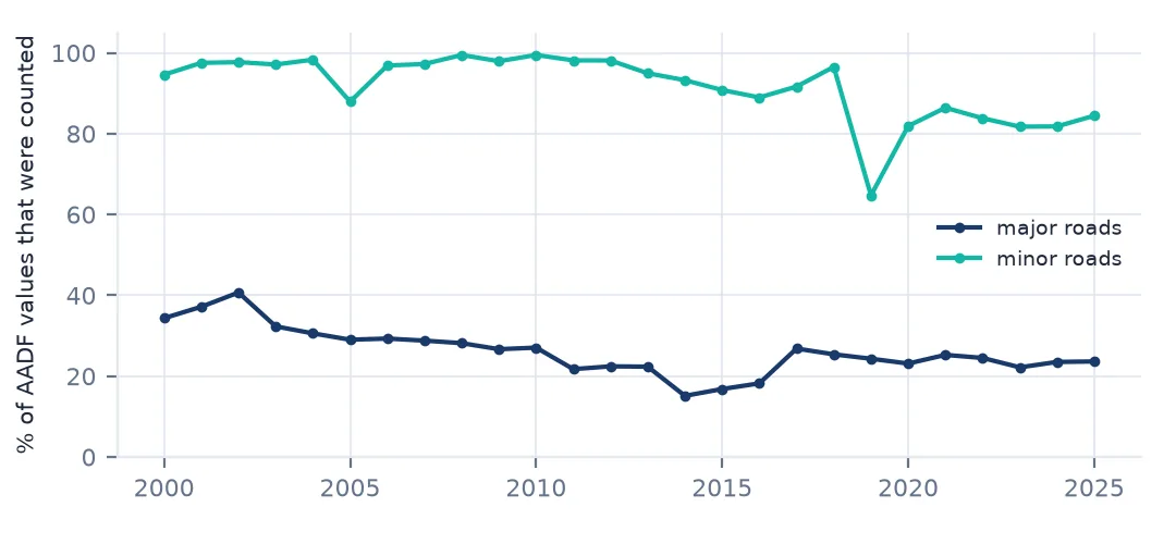
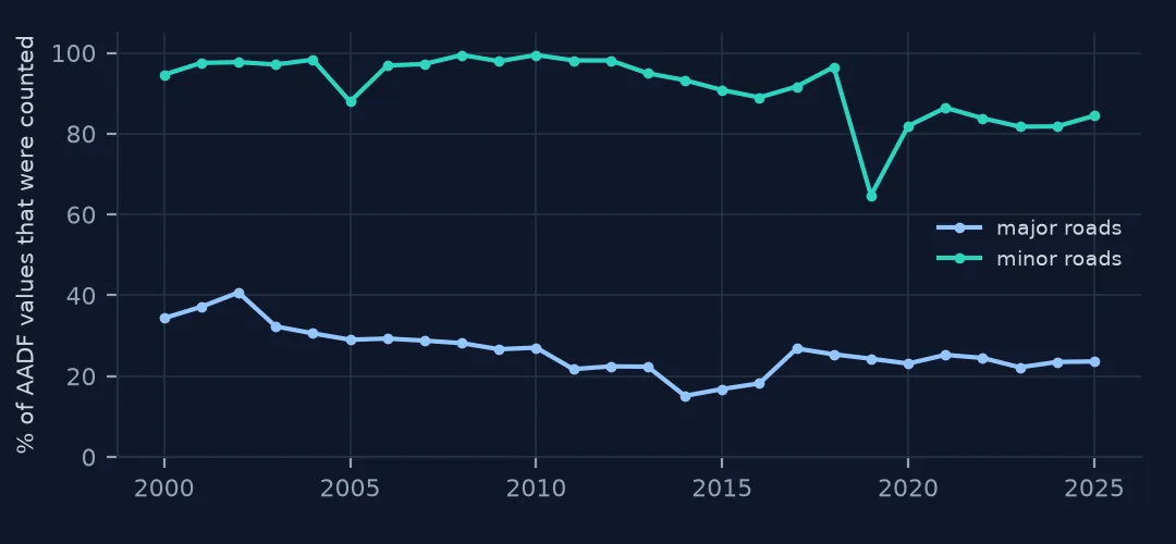
Manual counts — an enumerator at the roadside for twelve hours — make up 222,105 rows, automatic counters 9,553, and the rest are estimates of four kinds, mostly last year's figure grown by a regional factor. Major roads are counted far less often than minor ones in this file: 23.6% of major-road values in 2025 were counted. Annual average daily flow explained covers how a count becomes an annual figure.
3. Two sets of coordinates
import geopandas as gpd
from pyproj import Transformer

pts = aadf.drop_duplicates("count_point_id")
lon, lat = Transformer.from_crs(27700, 4326, always_xy=True).transform(pts.easting.values, pts.northing.values)
gap = np.hypot((lat - pts.latitude) * 111_320, (lon - pts.longitude) * 111_320 * np.cos(np.radians(pts.latitude)))
print(f"distance between the easting/northing and the latitude/longitude of each point: median {np.median(gap):.1f} m, max {gap.max():.1f} m")
gdf = gpd.GeoDataFrame(y, geometry=gpd.points_from_xy(y.easting, y.northing), crs=27700)
print(gdf.region_name.value_counts().to_string())
distance between the easting/northing and the latitude/longitude of each point: median 1.8 m, max 4.7 m
region_name
South East 2916
North West 2806
Scotland 2602
West Midlands 2132
London 2050
East of England 2021
South West 1993
Yorkshire and The Humber 1773
East Midlands 1723
Wales 1395
North East 923
Each point carries a British National Grid easting and northing and a latitude and longitude, and the two agree to within 4.7 m: either can be used. Build geometries from the easting and northing in EPSG:27700, which is metric and is what the rest of British open data uses.
4. Links on major roads, points on minor ones
print(aadf.groupby("road_type")[["link_length_km", "start_junction_road_name"]].apply(lambda g: g.notna().mean()).round(3).to_string())
print(y[y.road_type == "Major"].link_length_km.describe().round(1).to_string())
link_length_km start_junction_road_name
road_type
Major 1.0 0.999
Minor 0.0 0.000
count 17941.0
mean 2.9
std 4.0
min 0.1
25% 0.6
50% 1.5
75% 3.3
max 66.1
Major-road points represent a link between two junctions and carry its length; minor-road points stand for themselves and carry neither a length nor junction names. A median major link is 1.5 km long and the longest 66.1 km. Only major roads can therefore be turned into vehicle-kilometres (how).
5. Vehicle classes add up
hgv = ["HGVs_2_rigid_axle", "HGVs_3_rigid_axle", "HGVs_4_or_more_rigid_axle", "HGVs_3_or_4_articulated_axle",
       "HGVs_5_articulated_axle", "HGVs_6_articulated_axle"]
motor = ["two_wheeled_motor_vehicles", "cars_and_taxis", "buses_and_coaches", "LGVs", "all_HGVs"]
diff = (aadf[hgv].sum(axis=1) - aadf.all_HGVs).abs()
print(f"all_HGVs equals the six HGV columns: {(diff == 0).mean():.2%}; where not, off by {diff[diff > 0].median():.0f} "
      f"(max {diff.max():.0f}); share off, by year: {(diff > 0).groupby(aadf.year).mean().loc[[2010, 2014, 2015, 2025]].round(2).to_dict()}")
print(f"all_motor_vehicles equals the motor classes: {(aadf[motor].sum(axis=1) == aadf.all_motor_vehicles).mean():.2%}")
print(f"pedal cycles are not in all_motor_vehicles: share of cycles in 2025 traffic {y.pedal_cycles.sum() / (y.pedal_cycles.sum() + y.all_motor_vehicles.sum()):.2%}")
all_HGVs equals the six HGV columns: 76.14%; where not, off by 1 (max 6); share off, by year: {2010: 0.0, 2014: 0.43, 2015: 0.43, 2025: 0.44}
all_motor_vehicles equals the motor classes: 75.46%
pedal cycles are not in all_motor_vehicles: share of cycles in 2025 traffic 0.83%
From 2014 onwards the vehicle classes are rounded separately, so all_HGVs differs from the sum of its six axle classes in 43–44% of rows each year — by 1 vehicle typically and 6 at most. Use the published totals rather than re-adding the parts. Pedal cycles are counted but kept out of all_motor_vehicles; they are 0.83% of the traffic at 2025's count points.
The busiest points and one road
The data used on this page
The Department for Transport's road traffic statistics: annual average daily flows (AADF) for every count point in Great Britain, 2000–2025, in the release of 2 June 2026, saved on this site because DfT revises earlier years with each release. Contains public sector information licensed under the Open Government Licence v3.0.
from pathlib import Path

import numpy as np
import pandas as pd
import requests

Path("data").mkdir(exist_ok=True)
# DfT republishes the counts every June and revises earlier years; this is the release of 2 June 2026
# (live: https://storage.googleapis.com/dft-statistics/road-traffic/downloads/data-gov-uk/dft_traffic_counts_aadf.zip).
AADF = "dft-traffic-counts-aadf-2026-06-02.zip"
if not Path(f"data/{AADF}").exists():
    Path(f"data/{AADF}").write_bytes(requests.get(f"https://data.spatialworkflow.io/{AADF}", timeout=600).content)
aadf = pd.read_csv(f"data/{AADF}", low_memory=False)
print(f"{len(aadf):,} rows, {aadf.count_point_id.nunique():,} count points, {aadf.year.min()}-{aadf.year.max()}")
600,551 rows, 46,754 count points, 2000-2025
Example 1: the busiest count points
top = y.nlargest(5, "all_motor_vehicles")[["count_point_id", "road_name", "local_authority_name", "start_junction_road_name",
                                            "end_junction_road_name", "estimation_method", "all_motor_vehicles"]]
print(top.to_string(index=False))
count_point_id road_name local_authority_name start_junction_road_name end_junction_road_name estimation_method all_motor_vehicles
27923 M25 Hillingdon 14 LA Boundary Counted 212636
47876 M25 Surrey 13 14 Estimated 209610
7902 M25 Buckinghamshire 16 15 Estimated 208946
46050 M60 Salford 13 12 Counted 201196
57740 M25 Surrey 12 LA Boundary Counted 192857
The M25 west of London carries the most traffic in the file, 212,636 vehicles a day between junctions 14 and the boundary at Hillingdon; the M60 near Salford is the busiest outside the London area. Two of the top five are estimates.
Example 2: one road's profile
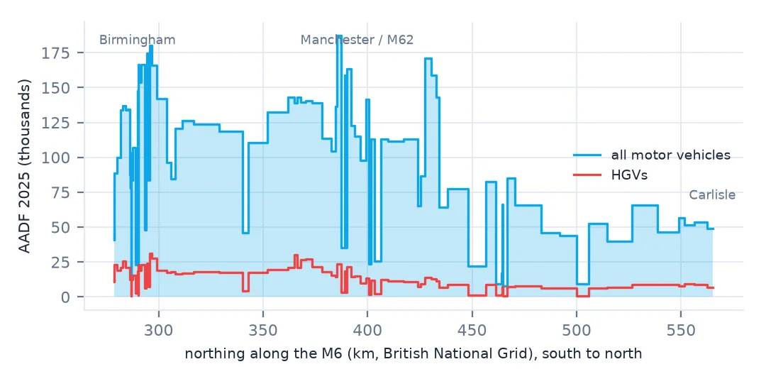
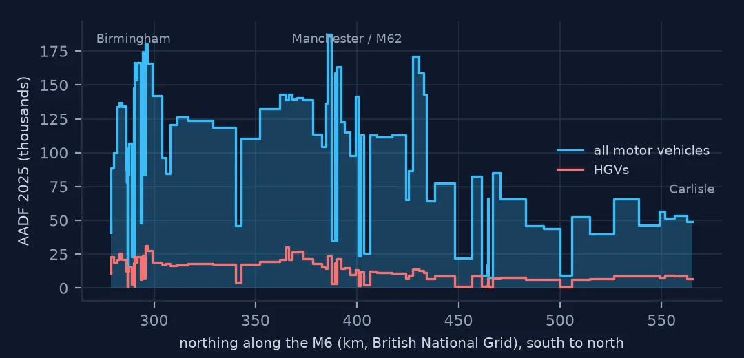
m6 = y[y.road_name == "M6"].sort_values("northing")
print(f"M6: {len(m6)} count points from {m6.northing.min():,} to {m6.northing.max():,} m north; "
      f"AADF from {m6.all_motor_vehicles.min():,} to {m6.all_motor_vehicles.max():,}")
print(m6.iloc[::12][["northing", "start_junction_road_name", "all_motor_vehicles", "all_HGVs"]].to_string(index=False))
M6: 99 count points from 278,790 to 565,313 m north; AADF from 7,828 to 187,521
northing start_junction_road_name all_motor_vehicles all_HGVs
278790 M1 46776 12125
286694 4 78075 12334
290730 5 153614 19215
302886 LA Boundary 142098 19165
366813 LA boundary 143072 21167
393300 21A (Junction 10 M62) 122662 14552
424766 29 65065 7366
465092 34 western spur 7828 520
552982 42 51683 9376
The M6 has 99 count points from the M1 junction near Rugby to Carlisle. Its traffic rises past Birmingham to 153,614 vehicles a day and falls to 7,828 at the western spur of junction 34 — the profile of one road read point by point.
A census of roads, mostly projected
The count points are a sample of the road network designed for national statistics. Every major-road link has a point, and each is counted in person every few years, with automatic counters on a few hundred. Minor roads are represented by a rotating sample of points. In the years between counts the figure is carried forward with growth factors from the counted links of the same kind and region.
That design makes the file excellent for "how much traffic is on this road" and for national totals, which is what it is built for, and treacherous for "how did traffic change here", because most rows in most years did not observe that. The guides on trends, estimated rows and changing samples deal with that.
Reading the file safely
- Filter on
estimation_methodwhen a question needs observed values. - Minor roads have no link length and no junction names; they are points.
- Road categories are codes: TM and PM motorways, TA and PA A roads, MB and MCU minor roads.
- Classes are rounded separately since 2014; use published totals.
- Pedal cycles are not motor vehicles in
all_motor_vehicles. - DfT revises earlier years with each June release; record which release you used.
Internal links
- Annual average daily flow explained — how a count becomes a yearly figure
- Traffic counts that all grow by the same percentage — what the estimated rows are
- How to turn traffic counts into vehicle-kilometres — using the link lengths
- How to map lorry traffic and freight corridors — the HGV columns on a map
FAQ
What is the busiest road in Britain by traffic count?
In the 2025 figures, the M25 between junction 14 and the Hillingdon boundary, at 212,636 vehicles a day.
Are DfT traffic counts real counts or estimates?
Mostly estimates: of 600,551 rows from 2000 to 2025, 222,105 are manual counts and 9,553 automatic counts; the rest are estimated, usually from the previous year's figure.