
Traffic Counts That All Grow by the Same Percentage: Estimated AADF
On this page
Problem statement
Compute each count point's year-on-year traffic change from the DfT file, look for the roads where traffic is growing fastest or falling, and something odd appears: whole regions of points change by exactly the same percentage, year after year, to the third decimal place. They are not measurements. More than half of all AADF values are the point's previous figure multiplied by a growth factor that DfT applies to every uncounted link of the same road type in the same region, so they carry no information about their own road.
This page shows how to recognise those rows, how old the counts behind them are, what happens to an analysis of local change that keeps them, and which rows to keep instead.
Quick answer
Compute each point's growth on the year before and look at how much it varies within a region, year and road category, split by the way the value was obtained:
a = aadf.sort_values(["count_point_id", "year"])
a["prev"] = a.groupby("count_point_id").all_motor_vehicles.shift()
a["growth"] = a.all_motor_vehicles / a.prev
ok = a.prev.gt(100) & (a.groupby("count_point_id").year.shift() == a.year - 1)
iqr = lambda s: s.quantile(0.75) - s.quantile(0.25)
spread = a[ok].groupby(["estimation_method_detailed", "year", "region_name", "road_category"]).growth.agg(iqr)
print(spread.groupby(level=0).median().round(4).to_string())
estimation_method_detailed
Automatic counter 0.0516
Dependent on a neighbouring counted link 0.0893
Dependent on an automatic counter on a neighbouring link 0.0152
Estimated from nearby links 0.0268
Estimated using AADF from previous year on this link 0.0041
Manual count 0.1197
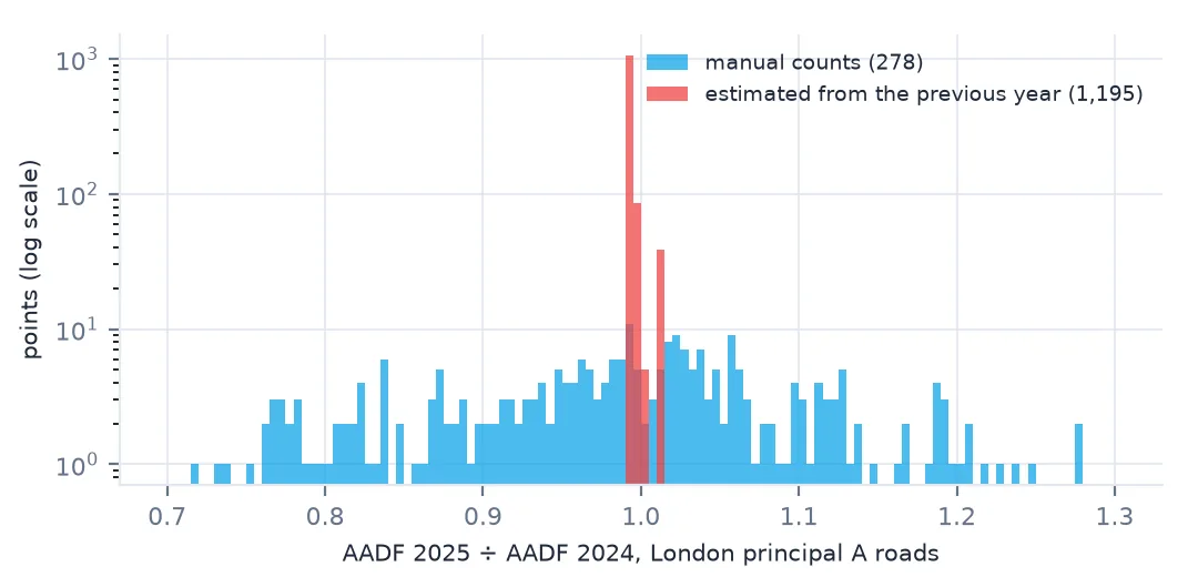
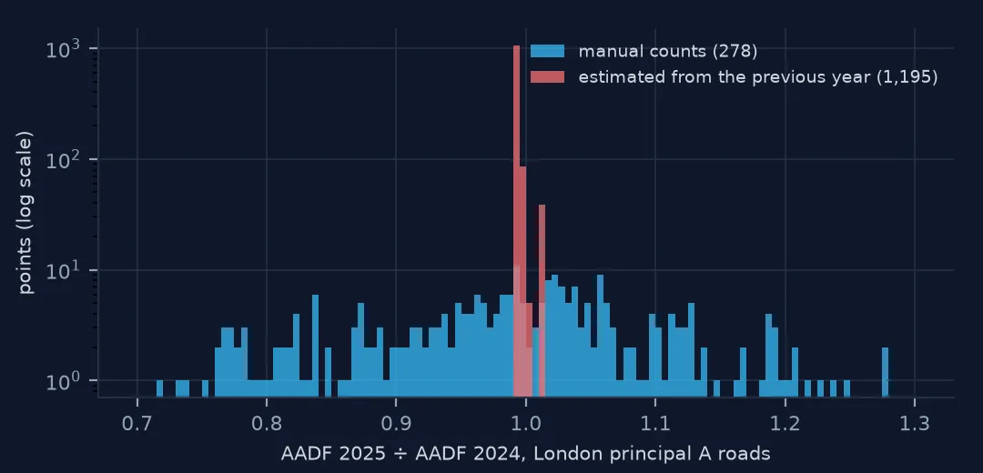
Within a region, year and road category, the growth of rows "estimated using AADF from previous year" varies with an interquartile range of 0.0041 — they all move together. Manual counts vary thirty times as much, 0.1197, as real roads do. Filter on estimation_method or estimation_method_detailed before asking anything about change at a place.
Recognising and dating estimates
1. Look at one region's estimated rows
ex = a[ok & (a.year == 2025) & (a.region_name == "London") & (a.road_category == "PA")]
print(ex.groupby("estimation_method_detailed").growth.describe(percentiles=[0.1, 0.5, 0.9]).round(4).to_string())
count mean std min 10% 50% 90% max
estimation_method_detailed
Automatic counter 178.0 1.0147 0.0766 0.8181 0.9560 0.9997 1.0920 1.3661
Dependent on a neighbouring counted link 30.0 0.9485 0.1355 0.6506 0.7679 0.9788 1.0775 1.1885
Dependent on an automatic counter on a neighbouring link 33.0 1.0137 0.0509 0.9348 0.9618 1.0107 1.0592 1.2126
Estimated from nearby links 58.0 0.9836 0.1680 0.0000 0.9465 0.9940 1.0648 1.4724
Estimated using AADF from previous year on this link 1195.0 0.9936 0.0037 0.9907 0.9915 0.9927 0.9952 1.0129
Manual count 278.0 0.9896 0.1287 0.4118 0.8186 0.9937 1.1345 1.4060
On London's principal A roads in 2025, 1,195 estimated values all grew by between 0.9915 and 0.9952 — a fall of half to one per cent — with a median of 0.9927. The 278 manual counts on the same kind of road ranged from 0.8186 to 1.1345 between their 10th and 90th percentiles. One group is a factor, the other is traffic.
2. How old is each estimate
counted = a[a.estimation_method == "Counted"].groupby("count_point_id").year.max().rename("last_counted")
y25 = a[a.year == 2025].join(counted, on="count_point_id")
y25["age"] = 2025 - y25.last_counted
print(y25.age.describe(percentiles=[0.25, 0.5, 0.75, 0.9]).round(1).to_string())
print(f"2025 values based on a count from 2015 or earlier: {(y25.age >= 10).mean():.1%}")
print(y25.groupby("road_type").age.median().to_string())
count 21036.0
mean 2.8
std 3.5
min 0.0
25% 0.0
50% 1.0
75% 5.0
90% 7.0
max 24.0
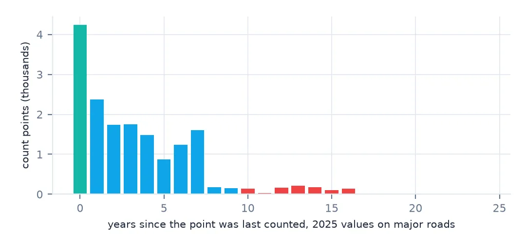
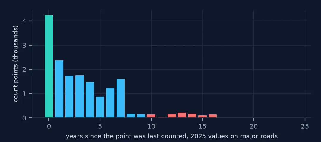
2025 values based on a count from 2015 or earlier: 4.6%
road_type
Major 2.0
Minor 0.0
For a median 2025 value the most recent count was a year earlier; a quarter of them are five or more years old, a tenth seven or more, and 4.6% rest on a count from 2015 or earlier. Major roads are counted less often than minor ones (median ages of 2 and 0 years) because minor-road points are mostly in the sample only in the years they are counted.
3. Growth hotspots that are not there
g = a[ok & a.year.between(2023, 2025)].groupby(["count_point_id", "estimation_method"]).growth.prod().reset_index()
top = g.sort_values("growth", ascending=False).head(200)
print("estimation method among the 200 fastest-growing points 2022-25:", top.estimation_method.value_counts().to_dict())
print("share of all points:", g.estimation_method.value_counts(normalize=True).round(3).to_dict())
estimation method among the 200 fastest-growing points 2022-25: {'Counted': 188, 'Estimated': 12}
share of all points: {'Estimated': 0.588, 'Counted': 0.412}
Rank points by growth from 2022 to 2025 and 188 of the 200 fastest are counted, although counted points are only 41.2% of the total. Estimated rows cannot show local growth, so a hotspot map built on all rows is a map of where counts happened — and among the counted rows the extremes are partly measurement noise from single-day counts.
4. Keep only rows with information of their own
own = a.estimation_method_detailed.isin(["Manual count", "Automatic counter"])
print(f"rows that are a measurement at that point and year: {own.mean():.1%}")
print(a[own].groupby("year").size().loc[[2000, 2010, 2019, 2020, 2025]].to_dict())
rows that are a measurement at that point and year: 38.6%
{2000: 7741, 2010: 8722, 2019: 13507, 2020: 7371, 2025: 7620}
Only 38.6% of all rows are a measurement at that point in that year: 7,620 in 2025, against 13,507 in 2019, the year of the enlarged minor-road sample. That is the data available for questions about local change.
Where the factors come from
The data used on this page
The Department for Transport's road traffic statistics: annual average daily flows (AADF) for every count point in Great Britain, 2000–2025, in the release of 2 June 2026, saved on this site because DfT revises earlier years with each release. Contains public sector information licensed under the Open Government Licence v3.0.
from pathlib import Path

import numpy as np
import pandas as pd
import requests

Path("data").mkdir(exist_ok=True)
# DfT republishes the counts every June and revises earlier years; this is the release of 2 June 2026
# (live: https://storage.googleapis.com/dft-statistics/road-traffic/downloads/data-gov-uk/dft_traffic_counts_aadf.zip).
AADF = "dft-traffic-counts-aadf-2026-06-02.zip"
if not Path(f"data/{AADF}").exists():
    Path(f"data/{AADF}").write_bytes(requests.get(f"https://data.spatialworkflow.io/{AADF}", timeout=600).content)
aadf = pd.read_csv(f"data/{AADF}", low_memory=False)
print(f"{len(aadf):,} rows, {aadf.count_point_id.nunique():,} count points, {aadf.year.min()}-{aadf.year.max()}")
600,551 rows, 46,754 count points, 2000-2025
Example 1: estimated growth tracks the regional factor
fac = a[ok & (a.estimation_method_detailed == "Estimated using AADF from previous year on this link")].groupby(
    ["year", "region_name", "road_category"]).growth.median().rename("factor")
cnt = a[ok & (a.estimation_method == "Counted")].groupby(["year", "region_name", "road_category"]).growth.median().rename("counted")
j = pd.concat([fac, cnt], axis=1).dropna()
print(f"{len(j)} region-year-category groups; correlation of estimated factor and counted median growth: {j.factor.corr(j.counted):.2f}")
print(j.loc[2020].groupby(level=1).median().round(3).to_string())
1357 region-year-category groups; correlation of estimated factor and counted median growth: 0.80
factor counted
road_category
MB 0.774 0.845
MCU 0.797 0.846
PA 0.770 0.810
PM 0.778 0.796
TA 0.705 0.763
TM 0.693 0.765
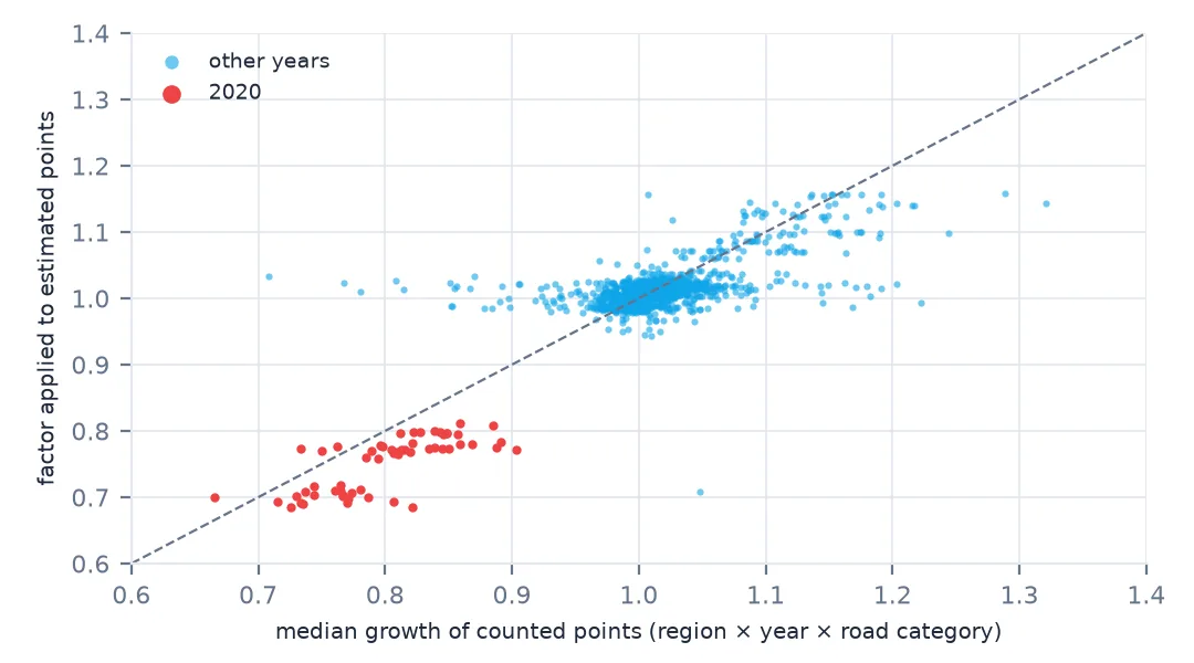
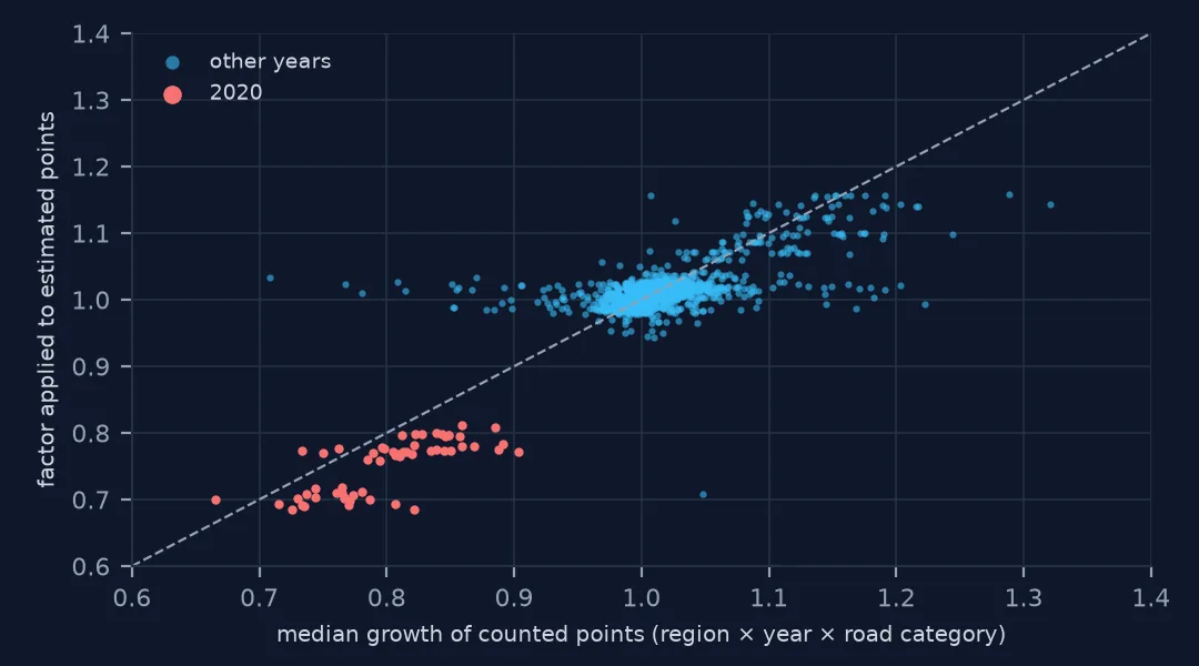
Across 1,357 region-year-category groups the estimated factor correlates at 0.80 with the median growth of counted points in the same group: the factors follow the counts, as intended, but not exactly. In 2020 they fell further than the counted medians in every road category — trunk motorways to 0.693 against 0.765 counted — probably because the factors also draw on DfT's automatic counters, which recorded the lockdown months that spring and autumn manual counts did not.
Example 2: neighbours copied, not counted
dep = a[ok & a.estimation_method_detailed.isin(["Dependent on a neighbouring counted link", "Estimated from nearby links"])]
print(dep.groupby("estimation_method_detailed").growth.agg(lambda s: iqr(s)).round(3).to_string())
estimation_method_detailed
Dependent on a neighbouring counted link 0.126
Estimated from nearby links 0.040
The two kinds of neighbour estimate differ: values "dependent on a neighbouring counted link" vary almost as much as counts (IQR 0.126), because they inherit that link's real change, while values "estimated from nearby links" vary little (0.040). Neither is a measurement of its own road.
Why the file is mostly projections
Counting every road every year would cost far more than the national statistics need. DfT counts each major-road link every few years and estimates it in between, using the change measured on counted links of the same type in the same region. For a national or regional total, which is what the figures are for, that works well: the estimates borrow strength from the counts and errors average out. For a single road in a single year, an estimate is a statement about its region, not about the road.
The file is honest about it: every row carries its estimation method. The mistake is only in not reading that column. Any question about change at a place — which roads grew, where traffic fell after a scheme, whether a junction got busier — should use counted rows, and should compare counts to counts.
Using estimated rows safely
- For totals and maps of a single year, estimated rows are fine; they are DfT's best figure.
- For change at a place, use counted rows only.
- Check the age of the last count before quoting a road's figure.
- Neighbour-based estimates inherit another link's change.
- 2020's factors fell further than counted medians; trends through 2020 differ by method.
Internal links
- Annual average daily flow explained — how the counted years are made
- How to measure traffic trends from count points that were actually counted — a trend without the estimates
- Average traffic drops when the survey adds minor roads — the other trap in the same file
FAQ
Why do so many UK traffic counts change by the same percentage each year?
Because they are not counts. 54.5% of AADF values are the previous year's figure multiplied by a growth factor shared by every uncounted link of the same road type in the region; within a group they vary by an interquartile range of 0.0041.
Which DfT traffic count rows are real measurements?
Rows whose estimation_method_detailed is "Manual count" or "Automatic counter": 38.6% of all rows from 2000 to 2025.