
Annual Average Daily Flow Explained: From a 12-Hour Count to a Year
On this page
Problem statement
An annual average daily flow is the number of vehicles that pass a point on an average day of the year, counting both directions, every day of the week and every hour. Almost none of that is observed. In Great Britain most AADF figures come from one person counting traffic at the roadside for twelve hours on one weekday in spring or autumn — or from no count at all that year. Everything else is expansion: from twelve hours to twenty-four, from a weekday to the week, from one month to the year.
This page explains how the Department for Transport turns a count into an AADF, using its published hourly counts alongside the AADF file: what the counts cover, how large the expansion is, how it varies by road and month, and how many published figures rest on no recent count at all.
Quick answer
Sum each manual count's twelve hours, join the published AADF for the same point and year, and divide — the ratio is the expansion that turned the one into the other:
day = raw.groupby(["count_point_id", "year"]).agg(count_12h=("all_motor_vehicles", "sum"), date=("count_date", "first"),
                                                   hours=("hour", "nunique"))
both = day.join(aadf.set_index(["count_point_id", "year"])[["all_motor_vehicles", "estimation_method", "road_category"]], how="inner")
both = both[(both.estimation_method == "Counted") & (both.hours == 12) & (both.count_12h > 0)]
both["expansion"] = both.all_motor_vehicles / both.count_12h
print(f"{len(both):,} counted point-years with a full 12-hour count")
print(both.expansion.describe(percentiles=[0.1, 0.5, 0.9]).round(3).to_string())
222,084 counted point-years with a full 12-hour count
count 222084.000
mean 1.145
std 0.112
min 0.667
10% 1.052
50% 1.131
90% 1.232
max 3.112
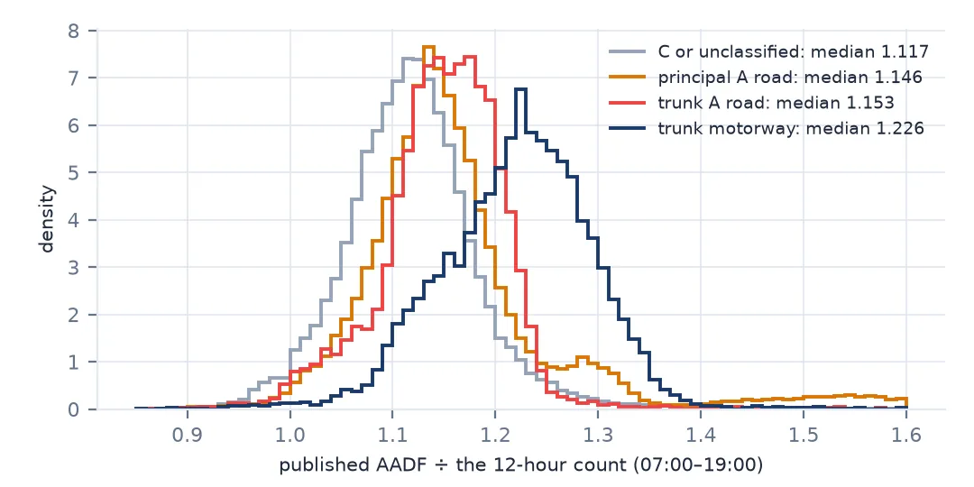
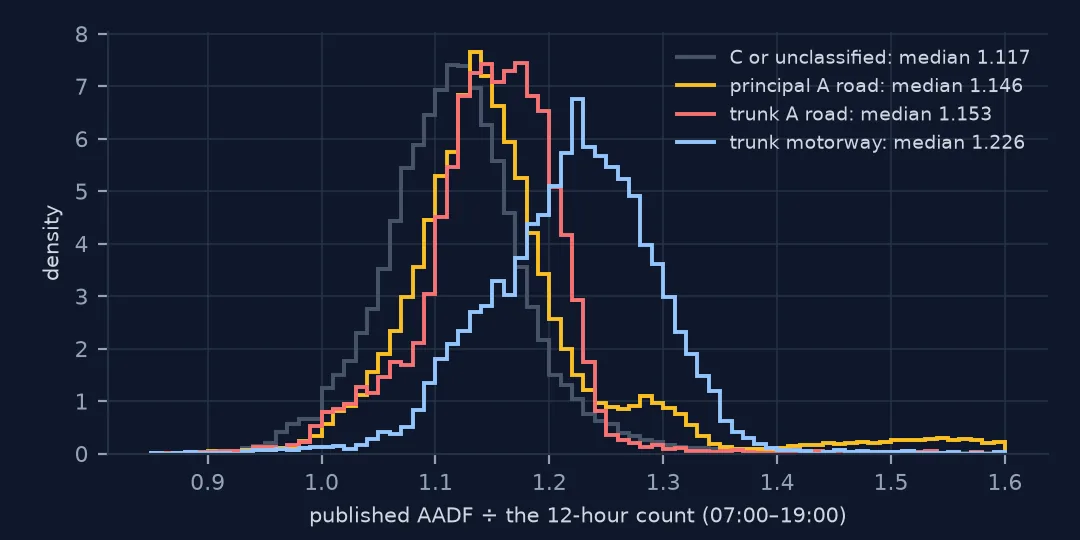
Across 222,084 counted point-years, the published AADF is a median 1.131 times the twelve-hour count, with the 10th and 90th percentiles at 1.052 and 1.232. A day's twelve hours carry most of its traffic; the expansion adds the night, the weekend and the season, and the three partly cancel — quiet nights and Sundays pull the average below a weekday, while the twelve missing hours push it up.
Twelve hours, one day, one year
1. What a manual count is
print("hours:", sorted(raw.hour.unique()))
print("weekday of count (0 = Monday):", raw.count_date.dt.dayofweek.value_counts().sort_index().to_dict())
print("month of count:", raw.count_date.dt.month.value_counts().sort_index().to_dict())
hours: [np.int64(0), np.int64(1), np.int64(3), np.int64(4), np.int64(5), np.int64(7), np.int64(8), np.int64(9), np.int64(10), np.int64(11), np.int64(12), np.int64(13), np.int64(14), np.int64(15), np.int64(16), np.int64(17), np.int64(18)]
weekday of count (0 = Monday): {0: 990912, 1: 1047948, 2: 1060956, 3: 1067148, 4: 1102536, 5: 12, 6: 120}
month of count: {3: 366024, 4: 598560, 5: 1000428, 6: 1084068, 7: 513492, 8: 600, 9: 957456, 10: 742320, 11: 6684}
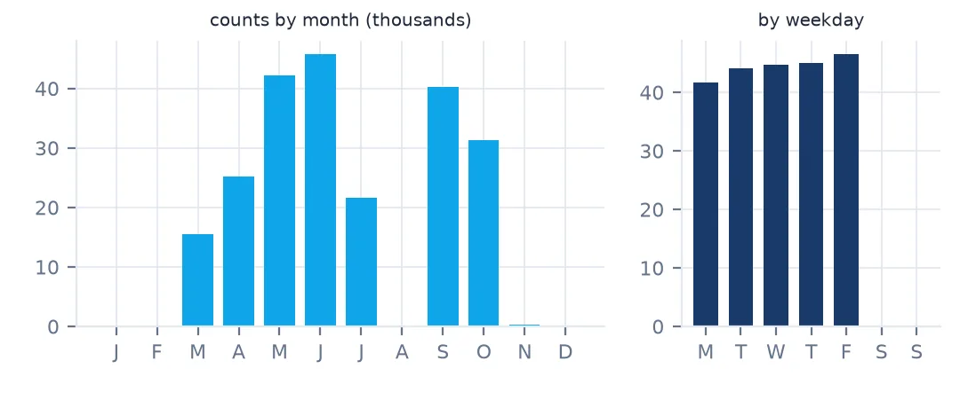
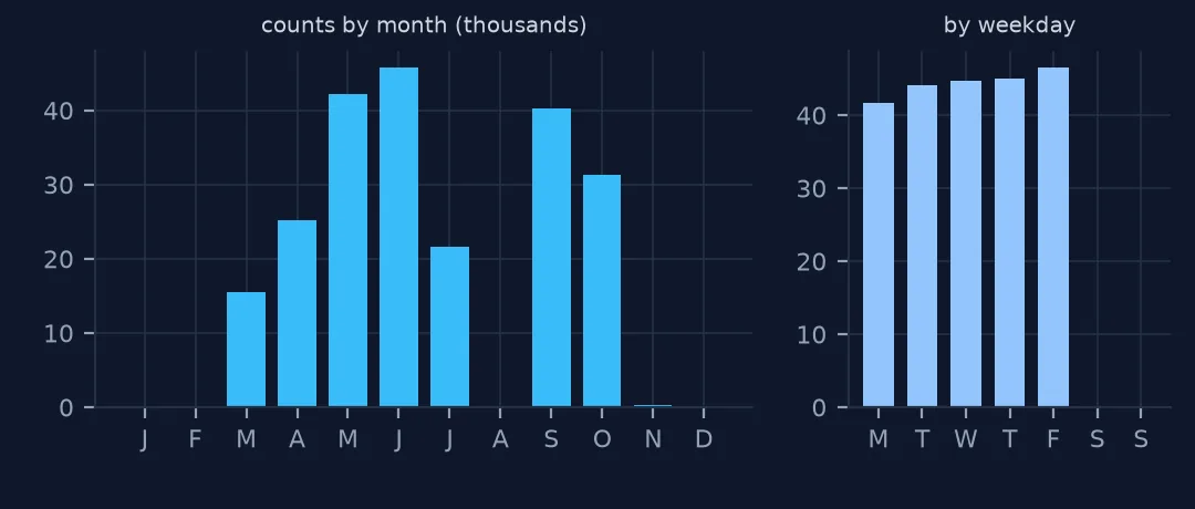
Manual counts run from 07:00 to 19:00 — the hours 7 to 18 in the file, with a handful of stray rows outside them — on weekdays only, and between March and October, avoiding August and the winter months when traffic is least typical. A count therefore samples the busiest, most regular part of the week.
2. From twelve hours to a day
print(both.groupby("road_category").expansion.median().round(3).to_string())road_category
MB 1.107
MCU 1.117
PA 1.146
PM 1.229
TA 1.153
TM 1.226
The expansion is larger on motorways (1.226–1.229) than on minor roads (1.107–1.117), because motorways carry much more of their traffic at night and at weekends: lorries overnight, long-distance trips on Saturdays and Sundays. A minor road's traffic is concentrated in the counted hours.
3. From one day to the year
both["month"] = both.date.dt.month
print(both.groupby("month").expansion.agg(["median", "size"]).round(3).to_string())
median size
month
3 1.137 15450
4 1.136 25234
5 1.116 42150
6 1.135 45725
7 1.136 21646
8 1.106 25
9 1.129 40299
10 1.135 31271
11 1.176 284
By month the median ratio moves only between 1.116 and 1.137. The seasonal factors DfT applies are designed to make a count in any month comparable with one in any other, and these medians show they do: the month a road was counted in hardly changes its annual figure.
4. Where there was no count
est = aadf.estimation_method_detailed.value_counts(normalize=True)
print((100 * est).round(1).to_string())
last = aadf[aadf.estimation_method == "Counted"].groupby("count_point_id").year.max()
y25 = aadf[aadf.year == 2025].set_index("count_point_id")
age = 2025 - last.reindex(y25.index)
print(f"2025 values whose most recent count was 10+ years earlier: {(age >= 10).mean():.1%}; never counted: {age.isna().mean():.1%}")
estimation_method_detailed
Estimated using AADF from previous year on this link 54.5
Manual count 37.0
Estimated from nearby links 5.1
Dependent on a neighbouring counted link 1.7
Automatic counter 1.6
Dependent on an automatic counter on a neighbouring link 0.1
2025 values whose most recent count was 10+ years earlier: 4.6%; never counted: 5.8%
Across all years, 37.0% of AADF figures come from a manual count and 1.6% from an automatic counter at that point; 54.5% are the previous year's figure grown by a factor, and the rest are borrowed from neighbouring links. For 2025, 4.6% of published values rest on a count at least ten years old, and 5.8% on no count in the whole 2000–2025 file.
One count and its annual average
The data used on this page
The Department for Transport's road traffic statistics: annual average daily flows (AADF) for every count point in Great Britain, 2000–2025, in the release of 2 June 2026, saved on this site because DfT revises earlier years with each release. Contains public sector information licensed under the Open Government Licence v3.0. The hourly manual counts behind them are DfT's raw-count file, 89 MB zipped, in the same release.
from pathlib import Path

import numpy as np
import pandas as pd
import requests

Path("data").mkdir(exist_ok=True)
# DfT republishes the counts every June and revises earlier years; this is the release of 2 June 2026
# (live: https://storage.googleapis.com/dft-statistics/road-traffic/downloads/data-gov-uk/dft_traffic_counts_aadf.zip).
AADF = "dft-traffic-counts-aadf-2026-06-02.zip"
if not Path(f"data/{AADF}").exists():
    Path(f"data/{AADF}").write_bytes(requests.get(f"https://data.spatialworkflow.io/{AADF}", timeout=600).content)
aadf = pd.read_csv(f"data/{AADF}", low_memory=False)
RAW = "dft_traffic_counts_raw_counts.zip"
if not Path(f"data/{RAW}").exists():
    # 89 MB; the release of 2 June 2026, which DfT replaces each June
    Path(f"data/{RAW}").write_bytes(requests.get(
        f"https://storage.googleapis.com/dft-statistics/road-traffic/downloads/data-gov-uk/{RAW}", timeout=900).content)
raw = pd.read_csv(f"data/{RAW}", parse_dates=["count_date"],
                  usecols=["count_point_id", "direction_of_travel", "year", "count_date", "hour", "road_category",
                           "road_type", "region_name", "pedal_cycles", "cars_and_taxis", "LGVs", "all_HGVs", "all_motor_vehicles"])
print(f"{len(raw):,} hourly rows from {raw.count_point_id.nunique():,} count points")
5,269,632 hourly rows from 43,401 count points
Example 1: an hourly count against its annual average
pick = both[both.road_category == "PA"].sort_values(["count_12h", "all_motor_vehicles"], kind="stable").index[len(both[both.road_category == "PA"]) // 2]
one = raw[(raw.count_point_id == pick[0]) & (raw.year == pick[1])]
print(f"count point {pick[0]}, counted {one.count_date.iloc[0]:%A %d %B %Y}, road category {one.road_category.iloc[0]}")
print(one.pivot_table(index="hour", columns="direction_of_travel", values="all_motor_vehicles", aggfunc="sum").to_string())
print(f"12-hour total {one.all_motor_vehicles.sum():,.0f}; published AADF {aadf.set_index(['count_point_id', 'year']).loc[pick, 'all_motor_vehicles']:,}")
count point 27511, counted Monday 27 June 2011, road category PA
direction_of_travel N S
hour
7 719.0 488.0
8 881.0 591.0
9 616.0 518.0
10 518.0 560.0
11 577.0 538.0
12 531.0 568.0
13 516.0 544.0
14 560.0 534.0
15 584.0 669.0
16 691.0 760.0
17 493.0 837.0
18 496.0 546.0
12-hour total 14,335; published AADF 15,527
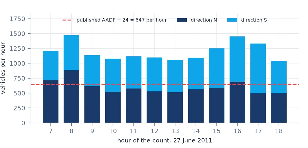
A principal A road counted on Monday 27 June 2011 shows the raw material: two directions, twelve hours, a morning peak northbound (881 vehicles between 8 and 9) and an evening peak southbound (837 between 17 and 18) — the tidal pattern of a commuter road. Its twelve hours sum to 14,335 vehicles; the published AADF for that year is 15,527, an expansion at the low end of the range.
Example 2: cyclists expand differently
cyc = raw.groupby(["count_point_id", "year"]).pedal_cycles.sum().rename("cycles_12h")
c = both.join(cyc).join(aadf.set_index(["count_point_id", "year"]).pedal_cycles.rename("cycles_aadf"))
c = c[c.cycles_12h >= 20]
print(f"cycle expansion factor: median {(c.cycles_aadf / c.cycles_12h).median():.3f}; motor vehicles: {c.expansion.median():.3f}")
cycle expansion factor: median 1.074; motor vehicles: 1.135
Cycles are expanded less than motor vehicles — a median 1.074 against 1.135 — because cycling is concentrated even more strongly in daylight weekday hours. That is an assumption built into the factors, not something the twelve-hour count measures, and it is weakest for leisure cycling at weekends.
An estimate built from three ratios
An AADF from a manual count is the count multiplied by three expansion factors, each taken from the continuous automatic counters that DfT runs on similar roads: the ratio of a full day to the counted twelve hours, of the average day of the week to that weekday, and of the annual average to that month. The factors differ by road type and region, which is why the overall ratio varies from road to road even though no single factor is large.
The consequences for anyone using the figures are practical. An AADF from a count is a good estimate of that year's traffic, with an uncertainty of several per cent from the single day sampled. An AADF in a year without a count is a projection of an older count, and the further it is from that count the less it says about the road and the more about the regional factor. And nothing in an AADF describes when traffic flows: for that, the hourly counts themselves are the data (hour-of-day profiles).
What the annual figure hides
- One weekday stands for the year. An unusual day — roadworks, an event — goes straight into the figure.
- Nights and weekends are modelled, from automatic counters on similar roads.
- Estimated years are projections. 5.8% of 2025 values rest on no count in the file.
- Cycle figures use their own factors, and are least reliable for leisure riding.
- Raw counts are per direction; AADF is both directions combined.
Internal links
- How to read UK road traffic counts — the AADF file itself
- How to build hour-of-day traffic profiles — the raw counts by hour
- Traffic counts that all grow by the same percentage — the estimated years
- How to measure cycling from road traffic counts — cycles in the same counts
FAQ
What does AADF mean in UK traffic data?
Annual average daily flow: the average number of vehicles passing a point on a day of the year, both directions combined. In the DfT data it is usually expanded from a single twelve-hour weekday count.
How is a 12-hour traffic count converted to AADF?
By multiplying it by factors for the missing hours, the day of the week and the month, taken from automatic counters. The combined ratio was a median 1.131 for counted points from 2000 to 2025.