How to Measure Traffic Trends from Count Points That Were Actually Counted

Problem statement

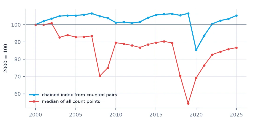
Has traffic on British roads grown since 2000? The DfT count file has a figure for every count point in every year it was in the sample, so the obvious answer is a line of the yearly median or mean. That line falls by almost half between 2000 and 2019 and then jumps, which says nothing about traffic: the set of count points changes from year to year, and most values in any year are estimates projected from an older count.

This page builds a traffic index from the count points that were actually counted in two consecutive years — the change at the same place, measured twice — and chains those year-on-year changes into a series. It then breaks the series down by road type and vehicle class, including the collapse of 2020.

Quick answer

Pair every counted year with the same point's counted previous year, take the median ratio each year, and multiply the ratios together:

a = aadf.sort_values(["count_point_id", "year"])
a["prev"] = a.groupby("count_point_id").all_motor_vehicles.shift()
a["prev_year"] = a.groupby("count_point_id").year.shift()
a["prev_counted"] = a.groupby("count_point_id").estimation_method.shift() == "Counted"
pair = a[(a.estimation_method == "Counted") & a.prev_counted & (a.prev_year == a.year - 1) & (a.prev > 0)]
step = pair.groupby("year").apply(lambda g: np.exp(np.log(g.all_motor_vehicles / g.prev).median()), include_groups=False)
index = step.cumprod() * 100
index.loc[2000] = 100
index = index.sort_index()
print(f"{len(pair):,} pairs of consecutive counted years")
print(index.loc[[2000, 2007, 2010, 2019, 2020, 2021, 2023, 2025]].round(1).to_string())

127,981 pairs of consecutive counted years
year
2000    100.0
2007    106.5
2010    101.2
2019    106.5
2020     85.4
2021     93.6
2023    102.3
2025    105.2

127,981 pairs of consecutive counted years give an index that rose to 106.5 by 2007, fell back to 101.2 by 2010 after the financial crisis, regained 106.5 by 2019, dropped to 85.4 in 2020 and has recovered to 105.2 in 2025. The median of geometric changes keeps one unusual point from moving a year.

Paired changes and a chained index

1. Why not the median of every point

naive = aadf.groupby("year").all_motor_vehicles.median()
print("median AADF of all points, 2000 = 100:", (100 * naive / naive.loc[2000]).loc[[2010, 2019, 2020, 2025]].round(1).to_dict())
print("count points per year:", aadf.groupby("year").size().loc[[2000, 2010, 2018, 2019, 2020, 2025]].to_dict())

median AADF of all points, 2000 = 100: {2010: 89.6, 2019: 54.4, 2020: 69.2, 2025: 86.7}
count points per year: {2000: 20009, 2010: 22257, 2018: 27543, 2019: 32903, 2020: 22373, 2025: 22334}

The median of all points, set to 100 in 2000, falls to 54.4 in 2019 and recovers to 86.7 in 2025 — almost entirely because the sample changed: 20,009 points in 2000, 32,903 in 2019, many of them added minor roads with little traffic. Average traffic drops when the survey adds minor roads takes that apart.

2. Pair each counted year with the one before it

print(pair.groupby("year").size().loc[[2001, 2010, 2019, 2020, 2021, 2025]].to_dict())
print(f"median year-on-year change, all pairs: {np.exp(np.log(pair.all_motor_vehicles / pair.prev).median()) - 1:+.2%}")

{2001: 4756, 2010: 4061, 2019: 5149, 2020: 3337, 2021: 4988, 2025: 4993}
median year-on-year change, all pairs: +0.75%

Each year has several thousand usable pairs — 3,337 in 2020, when counting was disrupted, and 4,061 to 5,149 in the other years shown. Across all of them the typical year-on-year change is +0.75%: small, which is why a few hundred unrepresentative points could swamp it in an unpaired comparison.

3. Chain the steps into an index

spread = pair.groupby("year").apply(lambda g: np.log(g.all_motor_vehicles / g.prev).quantile([0.25, 0.75]).diff().iloc[-1], include_groups=False)
print("spread (IQR of log change) in typical years and 2020:", spread.loc[[2015, 2019, 2020, 2021]].round(3).to_dict())

spread (IQR of log change) in typical years and 2020: {2015: 0.122, 2019: 0.115, 2020: 0.196, 2021: 0.155}

The spread of changes between points — the interquartile range of the log change — is 0.115–0.122 in ordinary years and widened to 0.196 in 2020. Traffic fell almost everywhere that year, but by very different amounts: some roads emptied and others barely changed.

4. Separate road types

by_type = {}
for rt, g in pair.groupby("road_type"):
    s = g.groupby("year").apply(lambda h: np.exp(np.log(h.all_motor_vehicles / h.prev).median()), include_groups=False)
    by_type[rt] = (s.cumprod() * 100).reindex(range(2001, 2026))
idx = pd.DataFrame(by_type)
print(idx.loc[[2010, 2019, 2020, 2025]].round(1).to_string())

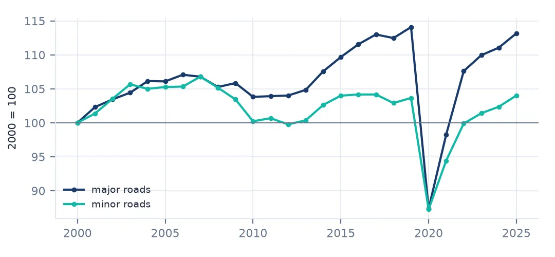
      Major  Minor
year              
2010  103.8  100.2
2019  114.1  103.7
2020   87.3   87.3
2025  113.2  104.0

Major and minor roads have different histories. Major roads ended 2019 at 114.1 and are at 113.2 in 2025; minor roads grew far less, to 103.7 and 104.0. The pooled index from the quick answer sits below both in 2019, which is the warning sign of a mix effect inside the chain: the share of major and minor pairs changes from year to year. A chained index should be built per stratum and combined with fixed weights, not pooled.

Estimated rows and vehicle types

The data used on this page

The Department for Transport's road traffic statistics: annual average daily flows (AADF) for every count point in Great Britain, 2000–2025, in the release of 2 June 2026, saved on this site because DfT revises earlier years with each release. Contains public sector information licensed under the Open Government Licence v3.0.

from pathlib import Path

import numpy as np
import pandas as pd
import requests

Path("data").mkdir(exist_ok=True)
# DfT republishes the counts every June and revises earlier years; this is the release of 2 June 2026
# (live: https://storage.googleapis.com/dft-statistics/road-traffic/downloads/data-gov-uk/dft_traffic_counts_aadf.zip).
AADF = "dft-traffic-counts-aadf-2026-06-02.zip"
if not Path(f"data/{AADF}").exists():
    Path(f"data/{AADF}").write_bytes(requests.get(f"https://data.spatialworkflow.io/{AADF}", timeout=600).content)
aadf = pd.read_csv(f"data/{AADF}", low_memory=False)
print(f"{len(aadf):,} rows, {aadf.count_point_id.nunique():,} count points, {aadf.year.min()}-{aadf.year.max()}")

600,551 rows, 46,754 count points, 2000-2025

Example 1: what the estimated rows would have said

a["prev_any"] = a.prev.notna() & (a.prev_year == a.year - 1) & (a.prev > 0)
est = a[a.prev_any & (a.estimation_method == "Estimated")]
step_est = est.groupby("year").apply(lambda g: np.exp(np.log(g.all_motor_vehicles / g.prev).median()), include_groups=False)
cmp = pd.DataFrame({"counted pairs": step - 1, "estimated rows": step_est - 1}).loc[[2015, 2019, 2020, 2021, 2022, 2025]]
print((100 * cmp).round(2).to_string())

      counted pairs  estimated rows
year                               
2015           1.55            2.06
2019           1.06            0.26
2020         -19.85          -22.94
2021           9.68            9.92
2022           7.28            7.04
2025           1.82            0.51

Year by year, the estimated rows move with the counted ones — they are grown with factors derived from counted links — but not identically: in 2019 the counted pairs grew 1.06% and the estimated rows 0.26%; in 2020 the estimates fell 22.94% against 19.85% counted. An index from all rows would partly be an index of DfT's factors. Traffic counts that all grow by the same percentage shows why.

Example 2: the pandemic by vehicle type

cls = {}
for col in ["cars_and_taxis", "LGVs", "all_HGVs", "pedal_cycles"]:
    sub = a.assign(pc=a.groupby("count_point_id")[col].shift())
    sub = sub[(sub.estimation_method == "Counted") & sub.prev_counted & (sub.prev_year == sub.year - 1) & (sub.pc > 0) & (sub[col] > 0)]
    s = sub.groupby("year").apply(lambda g: np.exp(np.log(g[col] / g.pc).median()), include_groups=False)
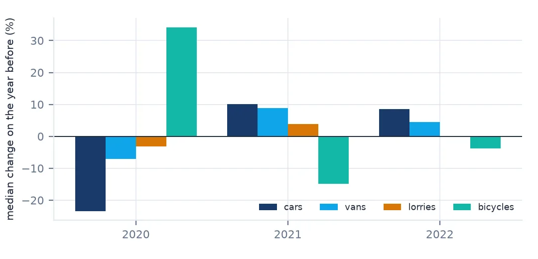
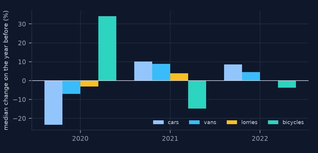
    cls[col] = (s.loc[2020:2022] - 1) * 100
print(pd.DataFrame(cls).round(1).to_string())

      cars_and_taxis  LGVs  all_HGVs  pedal_cycles
year                                              
2020           -23.4  -7.0      -3.1          34.1
2021            10.1   8.8       3.8         -14.9
2022             8.6   4.5       0.0          -3.8

In 2020 car traffic at counted points fell 23.4%, vans 7.0% and lorries only 3.1%, while cycling rose 34.1%. In 2021 cars recovered by 10.1% and cycling gave back 14.9%; by 2022 lorry traffic had stopped changing. Freight kept moving through the pandemic; commuting and leisure driving did not.

Why pairs, and why a chain

A trend needs the same thing measured at two times. The count file offers that only where a point was counted in both years; everywhere else either the point is new or old, or the value is an estimate that already contains an assumed trend. Pairing consecutive counted years keeps exactly the information about change and nothing else, and the median of the paired changes is robust to the odd roadworks year or misrecorded count.

Chaining multiplies the yearly changes into a series, so that each year contributes only what was observed between it and the year before. Its weakness is that errors accumulate along the chain and that the mix of pairs varies by year, which the per-road-type split exposes. Official road traffic statistics deal with the same problem with weighting by road length and with continuous automatic counters; this method is the transparent version that needs only the public file.

Pitfalls in traffic trends

• Never trend the median of all points. The sample changes.
• Never trend estimated rows. They follow the factors used to make them.
• Chain within strata. A pooled chained index can sit outside its parts.
• 2020 has fewer pairs and much wider spread; treat its step with care.
• The index is of flows at points, not of vehicle-kilometres, which also depend on the network.

Internal links

• Average traffic drops when the survey adds minor roads — why the naive median misleads
• Traffic counts that all grow by the same percentage — why estimated rows are left out
• How to measure cycling from road traffic counts — the same method for bicycles
• How to read UK road traffic counts — the file

FAQ

Has road traffic in Great Britain recovered since 2020?

At count points counted in consecutive years, traffic in 2025 stood at 105.2 on an index of 2000 = 100, against 106.5 in 2019 and 85.4 in 2020.

How much did traffic fall in 2020?

At counted points, car traffic fell 23.4% from 2019 to 2020, vans 7.0% and lorries 3.1%; cycling rose 34.1%.