
How to Build Hour-of-Day Traffic Profiles from Manual Counts
On this page
Problem statement
An annual average daily flow says how many vehicles use a road but not when. For congestion, noise, air quality, road safety or a cycle-lane case, the hour matters more than the day. Britain's road traffic statistics publish the hourly data behind the annual figures: every manual count since 2000, hour by hour and direction by direction, 5.3 million rows from 43,401 count points.
This page turns those counts into hour-of-day profiles for each kind of vehicle — cars, vans, lorries and bicycles — on major and minor roads, measures how tidal two-way roads are, and checks how the daily rhythm changed after 2020.
Quick answer
Sum the counts by road type and hour, then divide each vehicle class by its own total, so that the profile shows when each class travels rather than how many there are:
r = raw[raw.hour.between(7, 18)]
total = r.groupby(["road_type", "hour"])[["cars_and_taxis", "LGVs", "all_HGVs", "pedal_cycles"]].sum()
profile = total / total.groupby(level=0).transform("sum") * 100
print(profile.loc["Major"].round(1).T.to_string())
hour 7 8 9 10 11 12 13 14 15 16 17 18
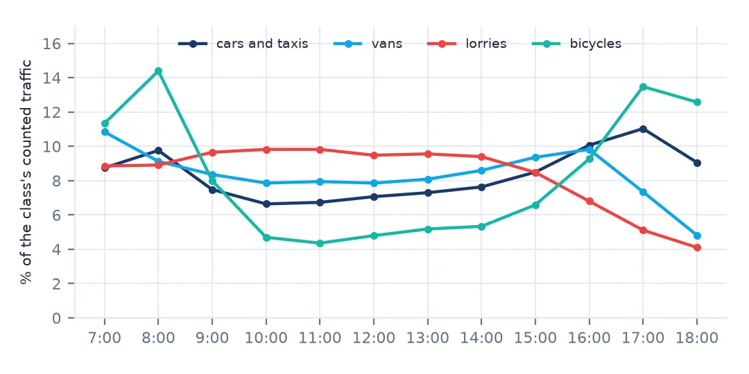
cars_and_taxis 8.7 9.8 7.5 6.6 6.7 7.1 7.3 7.6 8.5 10.1 11.0 9.1
LGVs 10.8 9.1 8.4 7.9 7.9 7.9 8.1 8.6 9.4 9.8 7.3 4.8
all_HGVs 8.9 8.9 9.7 9.8 9.8 9.5 9.6 9.4 8.5 6.8 5.1 4.1
pedal_cycles 11.3 14.4 8.0 4.7 4.4 4.8 5.2 5.3 6.6 9.3 13.5 12.6
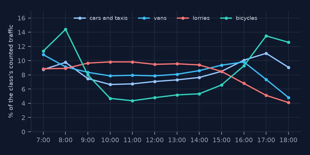
On major roads, cars peak in the evening (11.0% of their counted traffic between 17:00 and 18:00) with a smaller morning peak; vans peak earliest, at 07:00; lorries run at a steady 9–10% an hour from 07:00 to 15:00 and fall away after; bicycles have the sharpest double peak, 14.4% at 08:00 and 13.5% at 17:00. Each class has its own day.
Profiles, peaks and tides
1. Which counts to use
per = raw.groupby(["count_point_id", "year", "count_date"]).hour.nunique()
print("hours per count:", per.value_counts().head(4).to_dict())
print(f"counts from 2015 on: {(per.index.get_level_values('year') >= 2015).sum():,}")
hours per count: {12: 222092, 13: 8}
counts from 2015 on: 85,918
Every count but eight covers exactly twelve hours, so profiles can be built without reweighting partial counts. 85,918 counts are from 2015 onwards; using the whole archive back to 2000 is fine for shapes but mixes in older travel patterns.
2. Shares, not totals
peak = profile.groupby(level=0).apply(lambda p: p.droplevel(0).idxmax())
print(peak.to_string())
cars_and_taxis LGVs all_HGVs pedal_cycles
road_type
Major 17 7 10 8
Minor 17 16 9 17
The peak hours differ by road type too. On minor roads vans peak at 16:00 and cyclists in the evening rather than the morning; lorries on both kinds of road peak mid-morning. The evening peak of cars is the same everywhere.
3. Lorries keep office hours
for col in ["cars_and_taxis", "all_HGVs"]:
    p = profile.loc["Major", col]
    print(f"{col}: 07-10h {p.loc[7:9].sum():.1f}%, 10-16h {p.loc[10:15].sum():.1f}%, 16-19h {p.loc[16:18].sum():.1f}%")
cars_and_taxis: 07-10h 26.0%, 10-16h 43.9%, 16-19h 30.2%
all_HGVs: 07-10h 27.4%, 10-16h 56.6%, 16-19h 16.0%
On major roads 56.6% of counted lorry traffic falls between 10:00 and 16:00, against 43.9% of car traffic; only 16.0% of lorries travel in the evening peak hours, against 30.2% of cars. Freight is timed to avoid the peaks, which is why the HGV share of traffic is highest in the middle of the day.
4. Morning in, evening out
two = raw[raw.direction_of_travel.isin(["N", "S", "E", "W"])]
d = two.groupby(["count_point_id", "count_date", "direction_of_travel", "hour"]).all_motor_vehicles.sum().unstack("hour")
am = d.loc[:, 7:9].sum(axis=1); pm = d.loc[:, 16:18].sum(axis=1)
ratio = (am / pm).rename("am_pm").reset_index()
pairs = ratio.groupby(["count_point_id", "count_date"]).am_pm.agg(["min", "max", "size"])
pairs = pairs[pairs["size"] == 2]
print(f"{len(pairs):,} two-way counts; morning traffic as a share of evening traffic, median:")
print(f"  morning-heavy direction {pairs['max'].median():.2f}, evening-heavy direction {pairs['min'].median():.2f}")
print(f"counts where one direction carries at least 1.5x as much in the morning as in the evening: {(pairs['max'] >= 1.5).mean():.1%}")
216,892 two-way counts; morning traffic as a share of evening traffic, median:
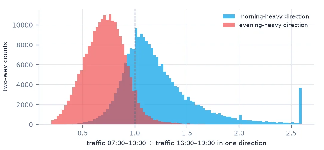
morning-heavy direction 1.15, evening-heavy direction 0.72
counts where one direction carries at least 1.5x as much in the morning as in the evening: 17.6%
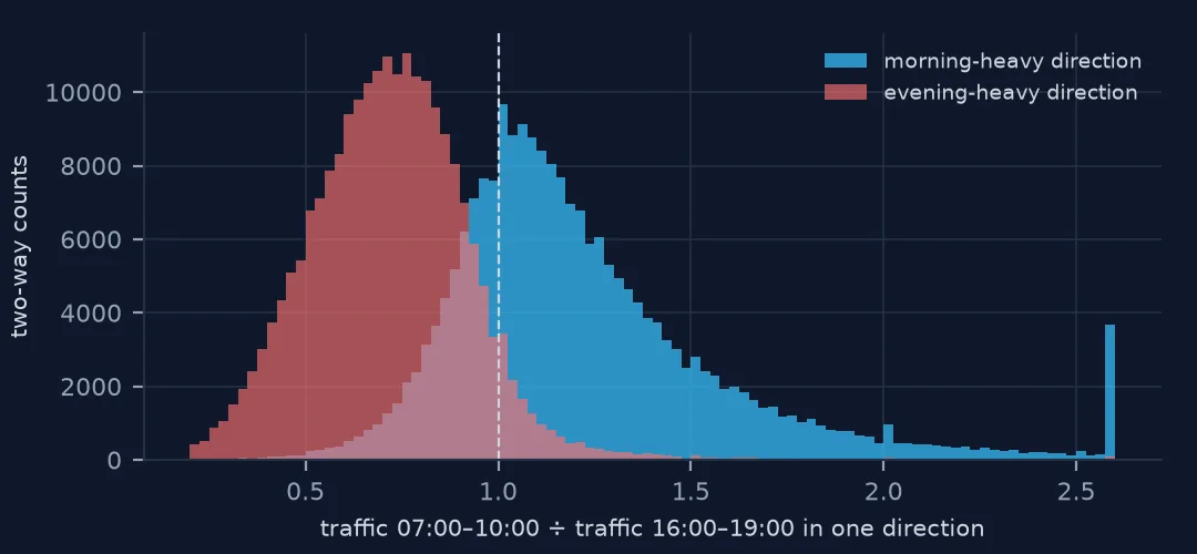
On 216,892 two-way counts, the morning-heavy direction carries 1.15 times its evening traffic in the morning peak and the evening-heavy direction 0.72 times: most roads are mildly tidal, with flows reversing between morning and evening. 17.6% are strongly tidal, one direction carrying at least half as much again in the morning as in the evening.
After 2020, and cyclists by road type
The data used on this page
The Department for Transport's road traffic statistics: the hourly manual counts behind every count point's annual figure, 2000–2025, in the release of 2 June 2026 (89 MB zipped), and the annual average daily flows from the same release, saved on this site. Contains public sector information licensed under the Open Government Licence v3.0.
from pathlib import Path

import numpy as np
import pandas as pd
import requests

Path("data").mkdir(exist_ok=True)
# DfT republishes the counts every June and revises earlier years; this is the release of 2 June 2026
# (live: https://storage.googleapis.com/dft-statistics/road-traffic/downloads/data-gov-uk/dft_traffic_counts_aadf.zip).
AADF = "dft-traffic-counts-aadf-2026-06-02.zip"
if not Path(f"data/{AADF}").exists():
    Path(f"data/{AADF}").write_bytes(requests.get(f"https://data.spatialworkflow.io/{AADF}", timeout=600).content)
aadf = pd.read_csv(f"data/{AADF}", low_memory=False)
RAW = "dft_traffic_counts_raw_counts.zip"
if not Path(f"data/{RAW}").exists():
    # 89 MB; the release of 2 June 2026, which DfT replaces each June
    Path(f"data/{RAW}").write_bytes(requests.get(
        f"https://storage.googleapis.com/dft-statistics/road-traffic/downloads/data-gov-uk/{RAW}", timeout=900).content)
raw = pd.read_csv(f"data/{RAW}", parse_dates=["count_date"],
                  usecols=["count_point_id", "direction_of_travel", "year", "count_date", "hour", "road_category",
                           "road_type", "region_name", "pedal_cycles", "cars_and_taxis", "LGVs", "all_HGVs", "all_motor_vehicles"])
print(f"{len(raw):,} hourly rows from {raw.count_point_id.nunique():,} count points")
5,269,632 hourly rows from 43,401 count points
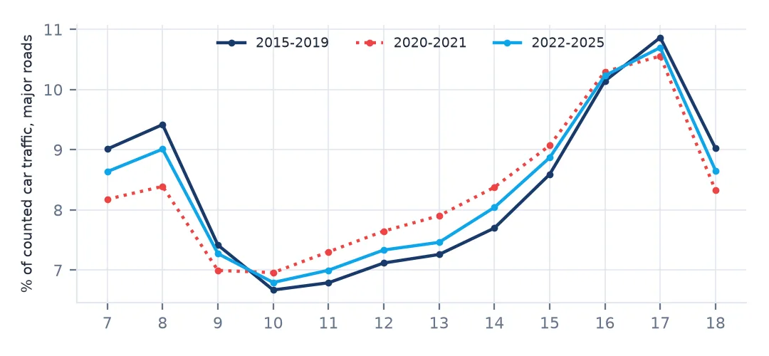
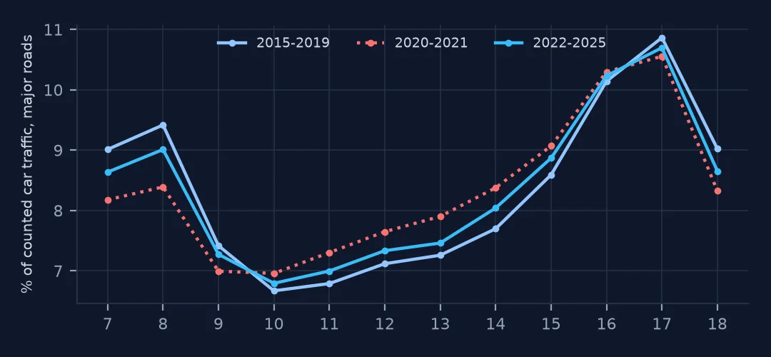
Example 1: the profile has changed since 2019
r["period"] = np.where(r.year <= 2019, "2015-2019", np.where(r.year >= 2022, "2022-2025", "2020-2021"))
r2 = r[(r.year >= 2015) & (r.road_type == "Major")]
pp = r2.groupby(["period", "hour"]).cars_and_taxis.sum()
pp = (pp / pp.groupby(level=0).transform("sum") * 100).unstack(0)
print(pp.loc[[7, 8, 9, 12, 15, 17, 18]].round(2).to_string())
period 2015-2019 2020-2021 2022-2025
hour
7 9.01 8.18 8.64
8 9.42 8.39 9.01
9 7.42 7.00 7.27
12 7.12 7.65 7.33
15 8.59 9.07 8.87
17 10.86 10.56 10.70
18 9.02 8.32 8.65
Car traffic's morning peak has not fully returned. At 08:00 the hour held 9.42% of the day's counted cars before 2020, 8.39% in 2020–2021 and 9.01% in 2022–2025, while the midday hours gained share. More flexible working would show up as a flatter morning like this, not a missing one.
Example 2: cycles by road type
print(profile.xs("pedal_cycles", axis=1).unstack(0).loc[[7, 8, 12, 17, 18]].round(1).to_string())road_type Major Minor
hour
7 11.3 9.7
8 14.4 12.2
12 4.8 5.7
17 13.5 12.7
18 12.6 10.5
Cyclists on major roads are the most commuter-like of all road users, with 14.4% of their counts at 08:00. On minor roads the morning peak is lower (12.2%) and the middle of the day busier (5.7% at noon).
Profiles as shares
A profile is a distribution over hours, and normalising each class to its own total is what makes the classes comparable: lorries are fewer than cars at every hour, but the shape shows when they travel. The same normalisation makes counts from different roads, years and seasons comparable, because a busy road and a quiet one contribute the same shape if their rhythms are the same.
The data's coverage sets the limits. Manual counts cover 07:00–19:00 on weekdays between March and October, so the profiles say nothing about nights, weekends or winter, and the evening "fall-off" for lorries is only the part of it before 19:00. For a full 24-hour week the source is DfT's automatic counters or a local authority's own loops; for the twelve weekday hours, these counts are the largest open sample there is.
Pitfalls with hourly counts
- Normalise each class by its own total before comparing shapes.
- Hours run 07:00–19:00 on weekdays; nights and weekends are not counted.
- Counts are per direction. Sum both for a two-way profile; keep them apart for tidal flows.
- Mixing decades mixes travel patterns. The morning peak changed after 2020.
- One count is one day. A single profile is noisy; average many.
Internal links
- Annual average daily flow explained — what the twelve hours become
- How to measure cycling from road traffic counts — cycles in the same counts
- How to separate commuting from leisure in bike-share trips — hourly profiles from trip data
- How to read UK road traffic counts — the annual file
FAQ
What time of day do lorries use UK roads most?
In the DfT manual counts, the middle of the day: 56.6% of counted lorry traffic on major roads falls between 10:00 and 16:00, against 43.9% of car traffic.
Has the morning rush hour returned since the pandemic?
Not fully. On major roads the 08:00 hour carried 9.42% of counted car traffic in 2015–2019 and 9.01% in 2022–2025.