Seismic Hazard Explained

Problem statement

"Seismic hazard" sounds like one number, and a hazard map prints one number per place, but behind it is a calculation over thousands of possible earthquakes: every fault and source zone that could shake a site, how often each produces earthquakes of each magnitude, and how strongly each would shake the site, with the scatter that real ground motions show. The result is a curve of ground motion against how often it is exceeded, and a design value is a point on that curve. Two further questions explain what the number means: which earthquakes it represents, and how that changes with the return period chosen.

This page uses the USGS 2018 National Seismic Hazard Model through its web services for three cities with different kinds of hazard, Los Angeles, Seattle and Memphis: it reads their hazard curves, converts between rates and probabilities, and disaggregates the hazard to find the magnitudes, distances and named sources that control it at two return periods.

Quick answer

Hazard is a curve; disaggregation says which earthquakes are behind a point on it:

for city in CITIES:
    s = summary(city, 2475)
    print(f"{city:>11}: PGA {s['PGA ground motion']:.2f} g at 2% in 50 years; mean M{s['m']:.1f} at {s['r']:.0f} km, epsilon {s['ε₀']:.2f}")

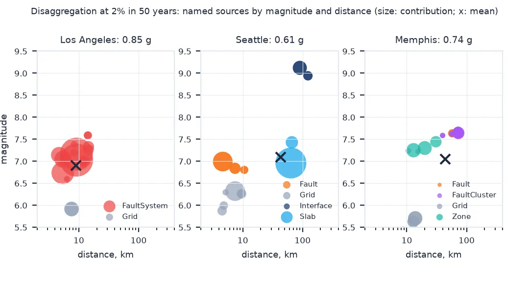
Los Angeles: PGA 0.85 g at 2% in 50 years; mean M6.9 at 9 km, epsilon 1.15
    Seattle: PGA 0.61 g at 2% in 50 years; mean M7.1 at 43 km, epsilon 1.29
    Memphis: PGA 0.74 g at 2% in 50 years; mean M7.0 at 44 km, epsilon 0.58

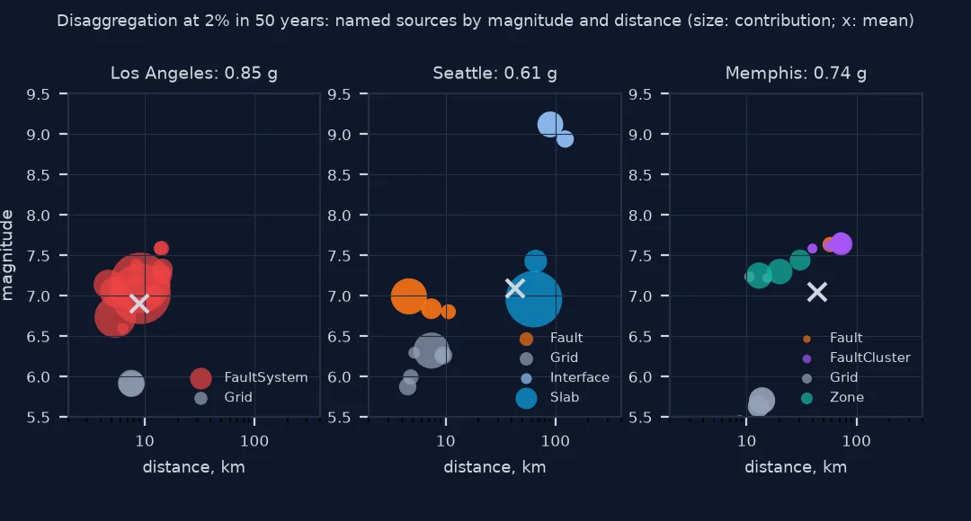
The three design values are similar, 0.61 to 0.85 g, but the earthquakes behind them are not. In Los Angeles the mean contributing earthquake is M6.9 at 9 km; in Seattle M7.1 at 43 km and in Memphis M7.0 at 44 km. Epsilon, the number of standard deviations above the median shaking that the hazard relies on, is 1.15 in Los Angeles and 1.29 in Seattle but 0.58 in Memphis.

Rates, return periods and probabilities, sources, design events

1. Rates, return periods and probabilities

A hazard curve gives annual rates. Convert a few points of one into return periods and probabilities over 50 years, which is how building codes state them:

xs, ys = curve("Seattle")
for target in (0.1, 0.2, 0.4, 0.8):
    rate = float(np.exp(np.interp(np.log(target), np.log(xs), np.log(ys))))
    print(f"Seattle, PGA > {target} g: {rate:.2e} a year = once in {1 / rate:,.0f} years = {1 - np.exp(-50 * rate):.1%} in 50 years")

Seattle, PGA > 0.1 g: 1.40e-02 a year = once in 71 years = 50.3% in 50 years
Seattle, PGA > 0.2 g: 4.87e-03 a year = once in 205 years = 21.6% in 50 years
Seattle, PGA > 0.4 g: 1.19e-03 a year = once in 839 years = 5.8% in 50 years
Seattle, PGA > 0.8 g: 1.76e-04 a year = once in 5,689 years = 0.9% in 50 years

In Seattle, PGA above 0.1 g has a return period of 71 years, a 50% chance in any 50 years. Each doubling of the ground motion makes it rarer by a factor of three to seven: 205 years for 0.2 g, 839 years for 0.4 g and 5,689 years for 0.8 g, under 1% in 50 years.

2. Which sources

Disaggregation splits the rate at the design ground motion among sources. List the largest named contributors for each city:

for city in CITIES:
    src = sources(city, 2475)
    single = src[src.type == "SINGLE"].nlargest(3, "contribution")
    print(f"{city}: " + "; ".join(f"{r['name']} {r.contribution:.1f}% (M{r.m:.1f}, {r.r:.0f} km)" for _, r in single.iterrows()))

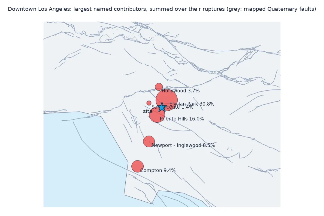
Los Angeles: Elysian Park (upper) (1) 19.7% (M6.7, 5 km); Elysian Park (upper) (1) 11.1% (M7.0, 5 km); Puente Hills (Los Angeles) [2] (1) 10.0% (M7.1, 5 km)
Seattle: Seattle (north) 14.8% (M7.0, 5 km); Cascadia (full, bottom) 7.6% (M9.1, 90 km); Seattle (middle) 4.8% (M6.8, 7 km)
Memphis: New Madrid - USGS (center, all) : R1-500-yr 5.8% (M7.6, 73 km); New Madrid - USGS (center, all) : R2-750-yr 3.9% (M7.6, 73 km); New Madrid - SSCn (BA-BL : RFT-S : NMN-S) : R2-270-yr 2.9% (M7.7, 72 km)

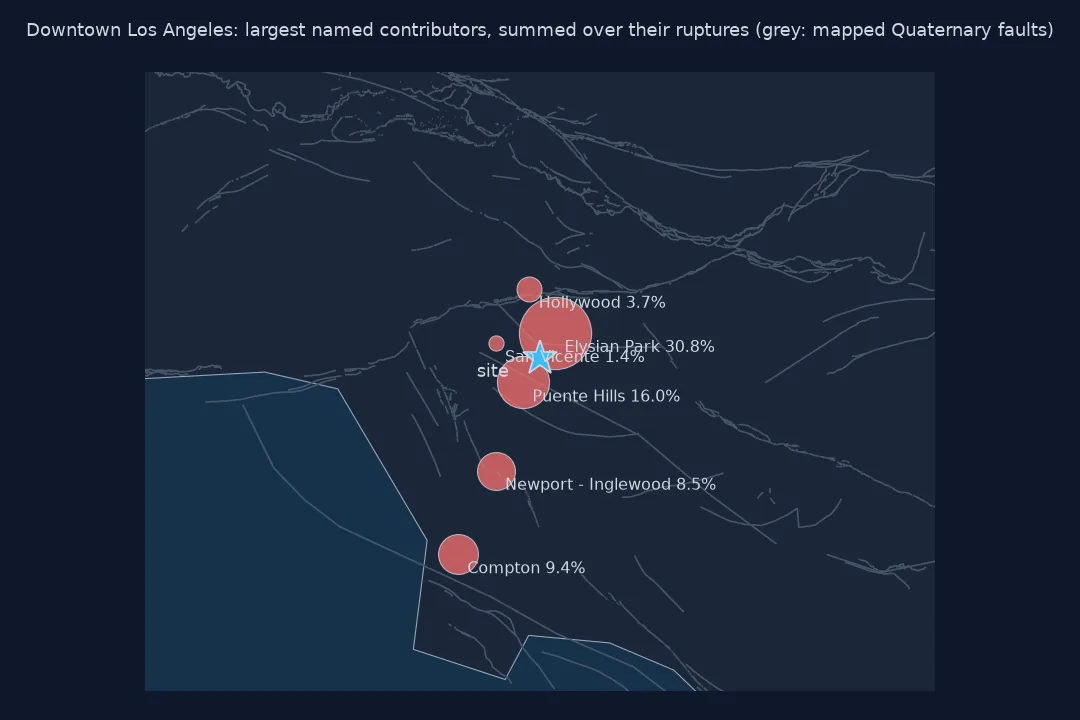
In Los Angeles the largest single contributors are blind thrusts under the city itself, the upper Elysian Park and Puente Hills faults, within 5 km of the site. In Seattle the Seattle fault, a few kilometres away, contributes most, and a full Cascadia subduction rupture, M9.1 at 90 km, appears second. In Memphis the contributions are spread over many logic-tree branches of the New Madrid source, each M7.6–7.7 at about 73 km, none above 6%.

3. The return period changes the earthquake

Rarer ground motions come from larger, closer earthquakes and from the stronger tail of the ground-motion scatter. Compare the disaggregation at 475 and 2,475 years:

for city in CITIES:
    a, b = summary(city, 475), summary(city, 2475)
    print(f"{city:>11}: 475 yr  PGA {a['PGA ground motion']:.2f} g, M{a['m']:.1f}, {a['r']:.0f} km, eps {a['ε₀']:.2f} | "
          f"2,475 yr PGA {b['PGA ground motion']:.2f} g, M{b['m']:.1f}, {b['r']:.0f} km, eps {b['ε₀']:.2f}")

Los Angeles: 475 yr  PGA 0.44 g, M6.8, 12 km, eps 0.56 | 2,475 yr PGA 0.85 g, M6.9, 9 km, eps 1.15
    Seattle: 475 yr  PGA 0.31 g, M7.0, 51 km, eps 0.74 | 2,475 yr PGA 0.61 g, M7.1, 43 km, eps 1.29
    Memphis: 475 yr  PGA 0.25 g, M6.9, 61 km, eps -0.14 | 2,475 yr PGA 0.74 g, M7.0, 44 km, eps 0.58

Going from 475 to 2,475 years roughly doubles the ground motion everywhere, but the contributing earthquakes change little in magnitude, by 0.1, and come closer: from 12 to 9 km in Los Angeles, 51 to 43 km in Seattle and 61 to 44 km in Memphis. Epsilon rises most: from 0.56 to 1.15 in Los Angeles and from -0.14 to 0.58 in Memphis. The rarer design level relies more on stronger-than-median shaking from the same kinds of earthquake.

Source types behind each city's hazard

The data used on this page

Hazard curves and disaggregations of peak ground acceleration for site class B/C (Vs30 760 m/s) from the USGS hazard web services for the 2018 conterminous US model. Coordinates are approximate city centres. Each request takes 20–30 seconds; the setup saves the responses.

import json
from pathlib import Path

import numpy as np
import pandas as pd
import requests

Path("data").mkdir(exist_ok=True)
CITIES = {"Los Angeles": (34.05, -118.25), "Seattle": (47.61, -122.33), "Memphis": (35.15, -90.05)}
BASE = "https://earthquake.usgs.gov/ws/nshmp/conus-2018/dynamic"
def get(kind, city, rp=None):
    lat, lon = CITIES[city]
    tag = f"_{rp}" if rp else ""
    p = Path(f"data/nshm2018_{kind}_{city.replace(' ', '_')}{tag}.json")
    if not p.exists():
        url = f"{BASE}/{kind}/{lon}/{lat}/760" + (f"/{rp}" if rp else "")
        r = requests.get(url, params={"imt": "PGA"} if rp else None, timeout=600)
        r.raise_for_status()
        p.write_text(r.text)
    d = json.loads(p.read_text())
    assert d["status"] == "success", d["response"]
    return d["response"]
def curve(city):
    c = next(h for h in get("hazard", city)["hazardCurves"] if h["imt"]["value"] == "PGA")
    v = next(d for d in c["data"] if d["component"] == "Total")["values"]
    xs, ys = np.array(v["xs"]), np.array(v["ys"])
    return xs[ys > 0], ys[ys > 0]
def _total(city, rp):
    return next(d for d in get("disagg", city, rp)["disaggs"][0]["data"] if d["component"] == "Total")
def summary(city, rp):
    out = {}
    for block in _total(city, rp)["summary"]:
        if block["name"] in ("Disaggregation targets", "Mean (over all sources)"):
            out.update({x["name"]: x["value"] for x in block["data"]})
    return out
def sources(city, rp):
    return pd.DataFrame(_total(city, rp)["sources"]).rename(columns={"ε": "eps"})
for city in CITIES:
    curve(city); summary(city, 475); summary(city, 2475)
print(f"{len(CITIES)} cities: hazard curves and disaggregations at 475 and 2,475 years")

3 cities: hazard curves and disaggregations at 475 and 2,475 years

The setup saves nine responses: a hazard curve and two disaggregations for each city, 85 seconds of server time on the first run.

Example 1: source types behind each city's hazard

Find the largest single entry of each source type in the disaggregation at 2,475 years:

for city in CITIES:
    src = sources(city, 2475)
    top = src.groupby("source").contribution.max().sort_values(ascending=False).head(4)
    print(f"{city}: largest contribution per source type: " + ", ".join(f"{k} {v:.0f}%" for k, v in top.items()))

Los Angeles: largest contribution per source type: FaultSystem 42%, Grid 8%
Seattle: largest contribution per source type: Slab 37%, Grid 15%, Fault 15%, Interface 8%
Memphis: largest contribution per source type: Grid 8%, Zone 8%, FaultCluster 6%, Fault 3%

The source types differ completely: Los Angeles's hazard comes from the California fault-system models, Seattle's from intraslab earthquakes, crustal faults, gridded seismicity and the Cascadia interface together, and Memphis's from many small entries of several types. The entries are logic-tree branches and overlap, so they cannot simply be summed to totals per type.

Cornell's sum

Probabilistic seismic hazard analysis, devised by Allin Cornell in 1968, rests on one sum. For every source, every magnitude it can produce and every distance at which it can produce it, multiply the annual rate of such earthquakes by the probability that one of them would exceed a ground-motion level at the site, according to a ground-motion model with its log-normal scatter; add everything up. That gives the annual rate of exceedance for the level, and repeating for many levels gives the hazard curve. Because the sum includes the scatter, a moderate earthquake nearby that happens to shake more strongly than its median, a positive epsilon, contributes alongside a large earthquake that shakes as expected.

Disaggregation runs the sum backwards. At a chosen ground motion it reports what fraction of the rate came from each magnitude, distance and epsilon, and from each named source. The result is the "design earthquake" that a single number hides: in one place a magnitude 7 on a fault a few kilometres away, in another a magnitude 9 on a subduction zone 100 km off the coast. That matters because shaking from those two would differ in duration and frequency content, even at the same PGA. And because rarer ground motions require bigger, closer earthquakes or more extreme scatter, the controlling earthquake changes with the return period.

Epsilon, mean against mode and logic trees

• Epsilon: the number of standard deviations above the median ground motion; values above 1 at long return periods mean the hazard leans on the tail of the ground-motion distribution.
• Mean versus mode: the mean magnitude and distance can describe an earthquake no source produces; the modal bin and the named sources are more concrete.
• Logic trees: the national model averages several fault models and ground-motion models; SET sources in the disaggregation are whole fault-system models.
• Time-independent: the national model assumes Poisson occurrence; time-dependent forecasts such as UCERF3's are separate products.

Internal links

• How to get seismic hazard curves in Python — the curves for five cities
• How to map seismic hazard and count exposed population in Python — the map
• How to estimate the probability of an earthquake from a catalogue in Python — rates and Poisson probabilities

FAQ

What is seismic hazard?

The probability that ground shaking at a site exceeds a given level in a given time, usually expressed as a hazard curve or as the ground motion with a stated probability of exceedance, such as 2% in 50 years.

What is the difference between hazard and risk?

Hazard is about the shaking; risk combines it with what is exposed and how vulnerable it is, to estimate losses.

What is seismic hazard disaggregation?

A breakdown of the hazard at one ground-motion level by the magnitude, distance, epsilon and source of the earthquakes that contribute to it.

Why does the controlling earthquake change with return period?

Because rarer, stronger ground motions can only be produced by larger or closer earthquakes, or by ground motions further above the median.