How to Estimate Population Exposure to Heat in Python

Problem statement

A surface temperature map shows where the city is hot. Heat policy needs where people are hot: how many residents live among the hottest surfaces, and in which districts. That means combining the heat map with a population grid — and the two come at very different resolutions (30 m heat, 100 m or 1 km population), which decides how the combination has to be done.

The result is a distribution: how the city's population is spread across the range of surface temperatures. Its upper tail — people living in the hottest tenth of the city — is the headline most programmes use.

Quick answer

Average the LST composite onto the population grid, then weight:

import io, zipfile, requests, numpy as np, rasterio
from rasterio.warp import reproject, Resampling
from rasterio.windows import from_bounds

name = "GHS_POP_E2020_GLOBE_R2023A_4326_30ss"
zipfile.ZipFile(io.BytesIO(requests.get(
    "https://jeodpp.jrc.ec.europa.eu/ftp/jrc-opendata/GHSL/GHS_POP_GLOBE_R2023A/"
    f"{name}/V1-0/tiles/{name}_V1_0_R5_C18.zip", timeout=600).content)).extractall("ghsl_es")
BOUNDS = (-3.85, 40.32, -3.55, 40.52)                           # the city of Madrid and its edge
with rasterio.open(f"ghsl_es/{name}_V1_0_R5_C18.tif") as src:
    win = from_bounds(*BOUNDS, src.transform)
    pop = np.clip(src.read(1, window=win), 0, None)
    ptf, pcrs = src.window_transform(win), src.crs

lst_on_pop = np.full(pop.shape, np.nan, dtype="float32")
with rasterio.open("madrid_lst_jja2023.tif") as src:            # from the composite guide
    reproject(rasterio.band(src, 1), lst_on_pop, dst_transform=ptf, dst_crs=pcrs,
              resampling=Resampling.average, src_nodata=np.nan, dst_nodata=np.nan)

ok = np.isfinite(lst_on_pop) & (pop > 0)
w, t = pop[ok], lst_on_pop[ok]
print(f"{w.sum():,.0f} people in {ok.sum():,} populated cells of ~0.7 km²")
print(f"area-weighted mean LST {t.mean():.1f} °C; population-weighted {np.average(t, weights=w):.1f} °C")
hot = t >= np.percentile(t, 90)
print(f"people in the hottest 10% of populated cells: {w[hot].sum():,.0f} ({w[hot].sum() / w.sum():.0%})")

4,285,905 people in 849 populated cells of ~0.7 km²
area-weighted mean LST 44.8 °C; population-weighted 43.1 °C
people in the hottest 10% of populated cells: 19,858 (0%)

The population-weighted mean says whether people live on hotter or cooler ground than the average cell, and in Madrid they live on cooler ground: 43.1 °C against 44.8 °C. The hottest tenth of populated cells holds 19,858 people, under half a percent of the 4.3 million — those cells are the sparsely populated fringe of dry farmland, airport and industry, the hottest surfaces at late morning.

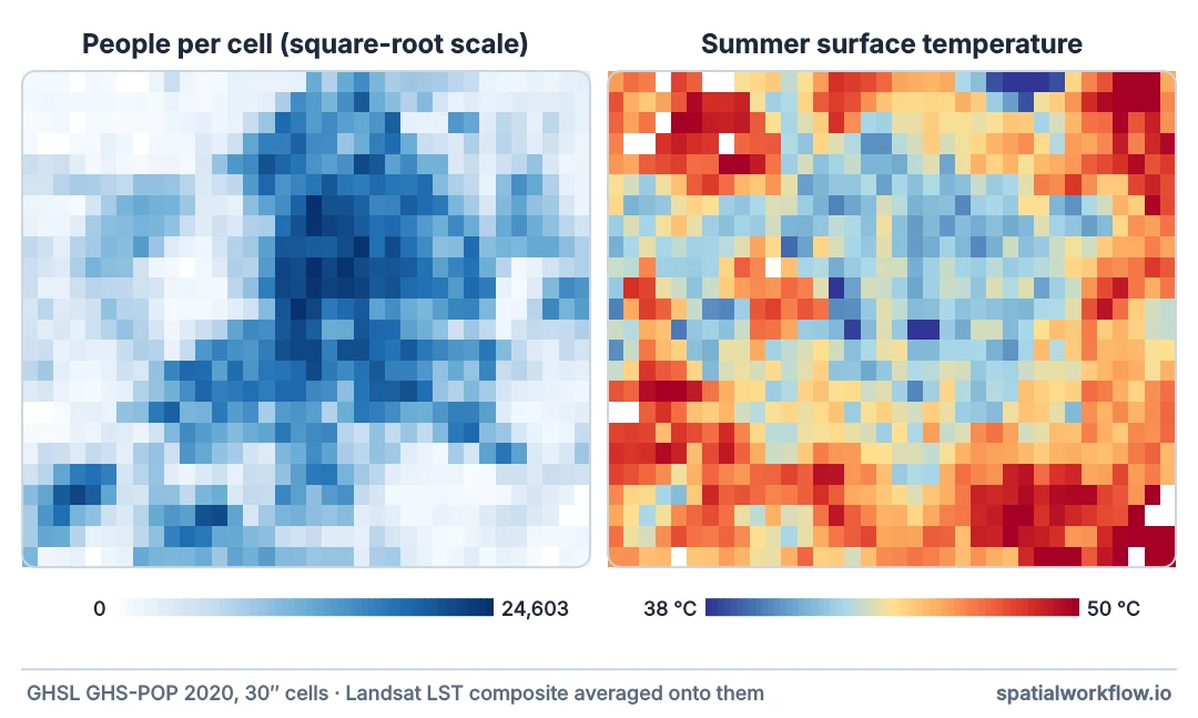
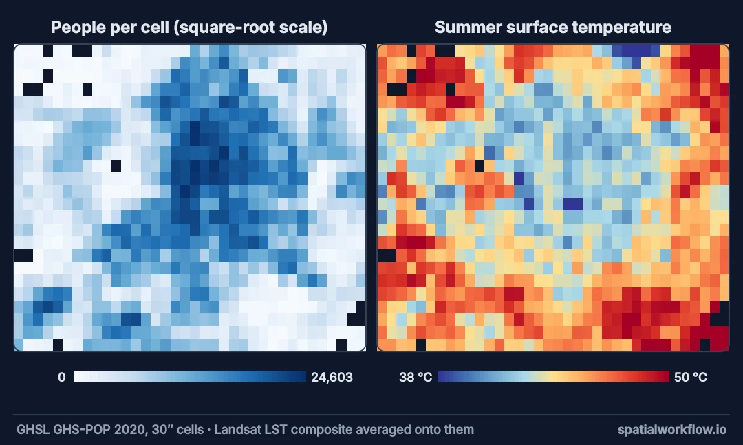
Heat on the population grid, valid cells, weighted statistics

1. Bring the heat map to the population grid

Average the 30 m LST within each population cell. Never interpolate population to 30 m: it is a count, and it would be invented at that resolution.

2. Keep cells with both people and valid LST

Cloud gaps and water leave cells without LST; unpopulated cells carry no exposure.

3. Compute weighted statistics

Population-weighted mean, percentiles and the share of people above thresholds.

4. Define "hot" relative to the city

The hottest decile of populated cells, or cells above the citywide 90th percentile. Absolute surface temperatures depend on the summer.

5. Break it down by district or group

Join to districts, age groups or deprivation indices to see who is most exposed — with the caveat that residential surface temperature is not personal exposure.

Madrid's population across surface temperature

The data used on this page

The summer 2023 land surface temperature composite of Madrid from the composite guide: the median of every Landsat 8 and 9 Collection 2 Level-2 scene from June to August 2023 on the Microsoft Planetary Computer with more than a fifth of the area clear, on a 30 m UTM 30N grid, with the count of clear observations as a second band. The setup rebuilds it if madrid_lst_jja2023.tif is missing.

import os

import numpy as np
import planetary_computer
import pystac_client
import rasterio
from rasterio.transform import from_origin
from rasterio.warp import Resampling, reproject, transform_bounds

if not os.path.exists("madrid_lst_jja2023.tif"):        # the composite guide's code, without the prints
    AOI = (-4.05, 40.20, -3.35, 40.65)
    DST_CRS = "EPSG:32630"
    x0, y0, x1, y1 = transform_bounds("EPSG:4326", DST_CRS, *AOI)
    x0, y1 = np.floor(x0 / 30) * 30, np.ceil(y1 / 30) * 30
    W, H = int(np.ceil((x1 - x0) / 30)), int(np.ceil((y1 - y0) / 30))
    DST_TF = from_origin(x0, y1, 30, 30)
    cat = pystac_client.Client.open("https://planetarycomputer.microsoft.com/api/stac/v1")
    items = [i for i in cat.search(collections=["landsat-c2-l2"], bbox=list(AOI),
                                   datetime="2023-06-01/2023-08-31").items()
             if i.properties["platform"] in ("landsat-8", "landsat-9") and i.properties["eo:cloud_cover"] < 60]

    def on_grid(item, asset):
        out = np.zeros((H, W), dtype="uint16")
        with rasterio.open(planetary_computer.sign(item.assets[asset].href)) as src:
            reproject(rasterio.band(src, 1), out, dst_transform=DST_TF, dst_crs=DST_CRS,
                      resampling=Resampling.nearest, src_nodata=0 if asset == "lwir11" else 1, dst_nodata=0)
        return out

    layers = []
    for it in sorted(items, key=lambda i: i.datetime):
        dn, qa = on_grid(it, "lwir11"), on_grid(it, "qa_pixel")
        t = np.where(dn == 0, np.nan, dn * 0.00341802 + 149.0 - 273.15)
        t[(((qa >> 1) & 1) | ((qa >> 3) & 1) | ((qa >> 4) & 1)) == 1] = np.nan
        if np.isfinite(t).mean() > 0.2:
            layers.append(t)
    stack = np.stack(layers)
    profile = {"driver": "GTiff", "height": H, "width": W, "count": 2, "dtype": "float32",
               "crs": DST_CRS, "transform": DST_TF, "nodata": np.nan, "compress": "deflate"}
    with rasterio.open("madrid_lst_jja2023.tif", "w", **profile) as dst:
        dst.write(np.nanmedian(stack, axis=0).astype("float32"), 1)
        dst.write(np.isfinite(stack).sum(axis=0).astype("float32"), 2)
        dst.set_band_description(1, "median LST °C, Landsat 8/9, Jun–Aug 2023")
        dst.set_band_description(2, "clear observations")
with rasterio.open("madrid_lst_jja2023.tif") as src:
    print(src.shape, src.crs, src.descriptions or "", f"median {np.nanmedian(src.read(1)):.1f} °C")

(1682, 1994) EPSG:32630 ('median LST °C, Landsat 8/9, Jun–Aug 2023', 'clear observations') median 46.9 °C

Example 1 — the population across surface temperature

edges = np.percentile(t, [0, 20, 40, 60, 80, 100])
for lo, hi in zip(edges[:-1], edges[1:]):
    m = (t >= lo) & (t <= hi)
    print(f"LST {lo:5.1f}–{hi:5.1f} °C: {m.mean():4.0%} of cells, {w[m].sum() / w.sum():4.0%} of people")

LST  36.6– 42.4 °C:  20% of cells,  35% of people
LST  42.4– 43.7 °C:  20% of cells,  37% of people
LST  43.7– 45.4 °C:  20% of cells,  19% of people
LST  45.4– 47.2 °C:  20% of cells,   7% of people
LST  47.2– 53.8 °C:  20% of cells,   2% of people

If people were spread evenly over the city's surfaces, each quintile of cells would hold a fifth of them. Here the two coolest quintiles hold 72% of the people and the two hottest only 9%: daytime surface heat and residents are concentrated in different places.

Example 2 — sensitivity to the population grid resolution

coarse_pop = pop[: pop.shape[0] // 3 * 3, : pop.shape[1] // 3 * 3].reshape(
    pop.shape[0] // 3, 3, pop.shape[1] // 3, 3).sum(axis=(1, 3))
coarse_lst = np.nanmean(lst_on_pop[: pop.shape[0] // 3 * 3, : pop.shape[1] // 3 * 3].reshape(
    pop.shape[0] // 3, 3, pop.shape[1] // 3, 3), axis=(1, 3))
okc = np.isfinite(coarse_lst) & (coarse_pop > 0)
print(f"~0.7 km² cells: population-weighted LST {np.average(t, weights=w):.2f} °C")
print(f"~6 km² cells:   population-weighted LST "
      f"{np.average(coarse_lst[okc], weights=coarse_pop[okc]):.2f} °C")
top_c = coarse_lst[okc] >= np.percentile(coarse_lst[okc], 90)
print(f"share of people in the hottest decile: fine {w[hot].sum() / w.sum():.0%}, "
      f"coarse {coarse_pop[okc][top_c].sum() / coarse_pop[okc].sum():.0%}")

~0.7 km² cells: population-weighted LST 43.08 °C
~6 km² cells:   population-weighted LST 43.29 °C
share of people in the hottest decile: fine 0%, coarse 0%

The weighted mean barely changes with resolution, and at both resolutions the hottest decile holds almost no one. In a city where the hottest cells are populated the tail is where resolution matters: coarser cells average hot blocks with cooler ones, and the people in the hottest places disappear into their surroundings.

Example 3 — does exposure follow density?

dens = w / 0.7                                                 # people per km², approximately
r = np.corrcoef(np.log1p(dens), t)[0, 1]
print(f"correlation between log population density and LST across populated cells: {r:.2f}")

correlation between log population density and LST across populated cells: -0.61

The denser the cell, the cooler its late-morning surface. Madrid's dense centre has street trees, courtyards and the shade of tall buildings; its thinly populated edge is dry grassland, runways and warehouse roofs, the hottest surfaces of all. That reverses the usual expectation, and it is a daytime surface result: at night, when stored heat in dense fabric matters most for sleep, the ranking can differ, and air temperature — not LST — is what residents feel.

Why weight by people, and why the tail matters

Why weight by population

Heat matters where people live. A hot airport apron or industrial estate raises a city's average LST without exposing many residents; a moderately hot, densely populated district may expose far more. Weighting by population turns a map of surfaces into a measure of residents' exposure.

Why the tail is the sensitive part

Averages are robust to resolution and grid choices; percentiles and threshold shares are not. The hottest places are small and dense, and their residents are identifiable only if both grids resolve them.

Why this is not personal exposure

Residents are placed at home; people spend their days elsewhere, indoors, where temperatures depend on buildings and cooling. Surface temperature is also not air temperature. The result locates where outdoor surfaces around homes are hottest, which is a planning target, not a health measurement.

GHSL tiles, night heat and vulnerability

• GHSL tiles are 10°; Madrid is in R5_C18 (40–50°N, 10°W–0°).
• 100 m population grids (GHSL, WorldPop) resolve more of the tail than 1 km ones.
• Night-time heat exposure needs night-time LST or air temperature models.
• Vulnerability: age, health and housing quality change who is harmed by the same exposure.
• Temporal mismatch: population 2020 and LST 2023 is normal; state both.

Internal links

• Heat exposure explained — hazard, exposure and vulnerability
• How to calculate population-weighted exposure — the same method for air pollution
• How to summarise LST by neighbourhood — district statistics
• How to build a summer LST composite — the heat input
• Exposure assessment explained — residential exposure and its limits
• Urban extent explained — which area to analyse

FAQ

How do I calculate how many people live in hot areas?

Average surface temperature onto the population grid and sum the population of cells above a threshold.

Should I resample population to the LST resolution?

No. Average LST onto the population grid; population is a count.

What counts as a hot area?

A relative threshold such as the citywide 90th percentile of populated cells is more comparable across years than an absolute one.

Why is population-weighted LST higher than the average?

Dense districts tend to be built-up and less green, with hotter surfaces.

Does grid resolution matter?

The mean hardly changes; the share of people in the hottest places does.

Is this the same as heat exposure for health?

No — it is residential surface heat, not personal air temperature exposure.