
Fixing Solar Farm Areas Computed in the Wrong Projection
On this page
Problem statement
The USPVDB's outlines come in EPSG:4326, longitude and latitude, and GeoPandas will compute .area on them without complaint, in square degrees, with only a warning. Reprojecting to Web Mercator, the projection of every web map, gives square metres that look plausible and are a third to twice too large across the lower 48, and several times too large in Alaska. The database already supplies the true array area as p_area, computed in an equal-area projection, which makes it the ideal check. This page computes the area every common way, shows which one matches, and deals with outlines made of many parts.
Quick answer
Compute the total area in degrees, Web Mercator and an equal-area projection, and compare each with p_area:
print(f"area in degrees (EPSG:4326): {pv.area.sum():.4f}")
for name, crs in [("Web Mercator", 3857), ("US Albers equal-area", 5070)]:
    a = pv.to_crs(crs).area
    print(f"{name}: total {a.sum() / 1e6:,.0f} km²; median ratio to p_area {(a / pv.p_area).median():.3f}")
area in degrees (EPSG:4326): 0.2841
Web Mercator: total 4,348 km²; median ratio to p_area 1.683
US Albers equal-area: total 2,853 km²; median ratio to p_area 1.000
In degrees the whole fleet covers 0.2841, a number with no unit worth using. Web Mercator gives 4,348 km², and the median facility comes out 1.683 times its p_area. The US Albers equal-area projection, EPSG:5070, gives 2,853 km² and a median ratio of 1.000: it reproduces the database's own areas.
Mercator, equal-area and multi-part outlines
1. Mercator grows with latitude
a3857 = pv.to_crs(3857).area
r = (a3857 / pv.p_area)
print(pv.assign(r=r).groupby(pd.cut(pv.ylat, [18, 30, 35, 40, 45, 50, 72])).r.median().round(3).to_string())
print(f"Alaska: {r[pv.p_state == 'AK'].median():.2f}")
ylat
(18, 30] 1.284
(30, 35] 1.450
(35, 40] 1.558
(40, 45] 1.827
(45, 50] 2.032
(50, 72] 5.417
Alaska: 5.42
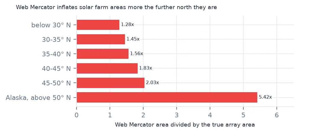
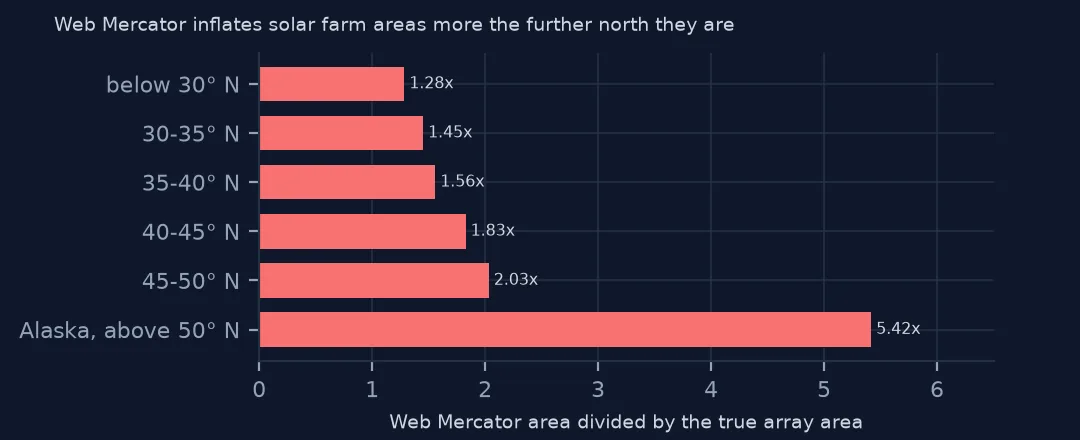
Mercator's error grows with latitude, as the square of its scale factor: by a median of 1.284 for facilities below 30° N, 1.558 between 35° and 40°, 2.032 between 45° and 50°, and 5.42 in Alaska. A map of solar land use computed in Web Mercator would show northern states using twice the land per megawatt of southern ones, purely from the projection.
2. Which equal-area projection
a5070 = pv.to_crs(5070).area
aak = pv.to_crs("+proj=aea +lat_1=55 +lat_2=65 +lat_0=50 +lon_0=-154 +datum=NAD83").area
print(f"5070 / p_area, worst: {(a5070 / pv.p_area).max():.3f} at {pv.loc[(a5070 / pv.p_area).idxmax(), 'p_name']}")
print(f"local Alaska Albers vs 5070 for Alaska's facilities: {(aak / a5070)[pv.p_state == 'AK'].round(4).tolist()}")
5070 / p_area, worst: 1.420 at North Rosamond Solar LLC
local Alaska Albers vs 5070 for Alaska's facilities: [1.0, 1.0]
EPSG:5070 agrees with p_area to within a hair everywhere except one record: North Rosamond Solar comes out 1.420 times its listed area, a multi-part outline where the listed area evidently covers only part of the geometry. For Alaska, an Albers projection centred on the state gives the same areas as 5070 to four decimals, so the national projection is good enough even there.
3. Multi-part outlines
parts = pv.explode(index_parts=False)
n = parts.groupby(level=0).size()
print(f"records: {len(pv):,}; parts: {len(parts):,}; most parts in one record: {n.max()} ({pv.loc[n.idxmax(), 'p_name']})")
c = pv.to_crs(5070).centroid
print(f"centroid outside its own outline: {(~c.within(pv.to_crs(5070).geometry)).sum()}")
records: 6,611; parts: 20,291; most parts in one record: 126 (Oxbow Solar 1)
centroid outside its own outline: 1345
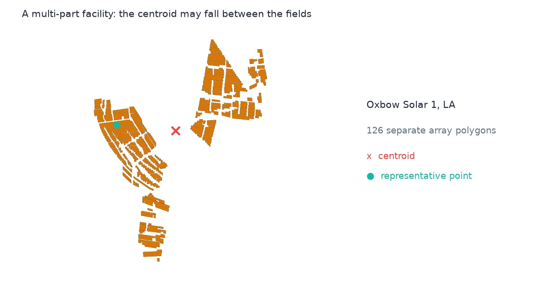
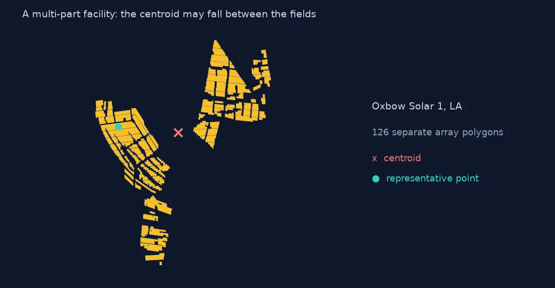
The 6,611 records explode into 20,291 polygons; Oxbow Solar 1 alone has 126 parts. Area works on the whole multipolygon, but the centroid does not: 1,345 facilities have a centroid outside their own outline, usually between separate fields. Use representative_point() or the database's own ylat and xlong when a point must lie on the facility.
One facility, every way
The data used on this page
The US Geological Survey and Lawrence Berkeley National Laboratory's US Large-Scale Solar Photovoltaic Database (USPVDB), version 4.0 of 14 April 2026 (Fujita and others, doi:10.5066/P9IA3TUS), public domain, as GeoJSON with the metadata and changelog from the download. USGS replaces the files at the same address with each version, so version 4.0 was saved on this site on 28 October 2026. Capacities are megawatts, areas square metres of panels and inverters.
from pathlib import Path
import zipfile

import geopandas as gpd
import numpy as np
import pandas as pd
import requests

Path("data").mkdir(exist_ok=True)
# USGS/LBNL US Large-Scale Solar Photovoltaic Database (USPVDB) version 4.0 of April 2026 (doi:10.5066/P9IA3TUS),
# array outlines as GeoJSON, with the Census Bureau's 2024 counties and states. Saved 28 October 2026: each new
# version replaces the files at the same address.
# Live: https://energy.usgs.gov/uspvdb/assets/data/uspvdbGeoJSON.zip
ARCHIVE = "usgs-uspvdb-v4-0-2026-10-28.zip"
if not Path(f"data/{ARCHIVE}").exists():
    Path(f"data/{ARCHIVE}").write_bytes(requests.get(f"https://data.spatialworkflow.io/{ARCHIVE}", timeout=600).content)
Z = zipfile.ZipFile(f"data/{ARCHIVE}")
for f in ["uspvdb_v4_0_20260414.geojson", "cb_2024_us_county_20m.zip", "cb_2024_us_state_20m.zip"]:
    if not Path(f"data/{f}").exists():
        Path(f"data/{f}").write_bytes(Z.read(f))
pv = gpd.read_file("data/uspvdb_v4_0_20260414.geojson")
print(f"USPVDB 4.0: {len(pv):,} solar facilities, {pv.p_cap_ac.sum():,.0f} MW AC")
USPVDB 4.0: 6,611 solar facilities, 131,574 MW AC
Example 1: one facility, every way
f = pv[pv.p_name == "Gemini Solar"]
for name, crs in [("degrees", None), ("Web Mercator", 3857), ("UTM 11N", 32611), ("US Albers", 5070)]:
    a = f.area.iloc[0] if crs is None else f.to_crs(crs).area.iloc[0]
    print(f"{name}: {a:,.6f}" if crs is None else f"{name}: {a / 1e6:.2f} km²")
print(f"p_area: {f.p_area.iloc[0] / 1e6:.2f} km²")
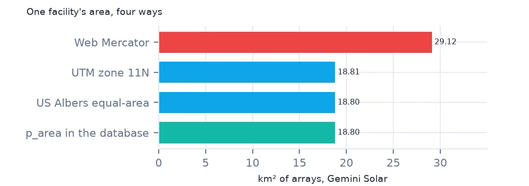
degrees: 0.001890
Web Mercator: 29.12 km²
UTM 11N: 18.81 km²
US Albers: 18.80 km²
p_area: 18.80 km²
For Gemini Solar in Nevada, the largest facility, the area in degrees is 0.001890; Web Mercator gives 29.12 km²; UTM zone 11N gives 18.81 km²; and US Albers 18.80 km², the listed p_area. A local UTM zone is as good as an equal-area projection for a single facility, but only within its own zone.
Internal links
- Solar farm land use — what the correct areas show
- Choosing a projected CRS for area — the general problem
- Reading the database — the outlines and points
- Area and distance in GeoPandas — the basic calculations