
How Much Land Do Solar Farms Use? Capacity per Area in Python
On this page
Problem statement
How much land a solar farm needs is one of the most argued questions about renewable energy, and the answer depends on what is measured. The USPVDB's p_area is the area of the panel arrays and inverters only, drawn from imagery, without fences, roads or setbacks, so it gives the core footprint of every facility of a megawatt or more. This page turns it into megawatts per square kilometre and acres per megawatt, compares tracking and fixed arrays and the years they were built, and looks at the records the database itself flags as implausible.
Quick answer
Divide DC capacity by array area for the whole fleet and for each facility, and express it in the acres per megawatt AC that planners use:
dens = pv.p_cap_dc / (pv.p_area / 1e6)                 # MW DC per km² of array
print(f"all facilities: {pv.p_cap_dc.sum() / (pv.p_area.sum() / 1e6):.1f} MW DC per km² of array; median facility {dens.median():.1f}")
acres_per_mw = (pv.p_area / 4046.86) / pv.p_cap_ac
print(f"acres of array per MW AC: median {acres_per_mw.median():.2f}; middle half {acres_per_mw.quantile(0.25):.2f}-{acres_per_mw.quantile(0.75):.2f}")
all facilities: 57.1 MW DC per km² of array; median facility 66.6
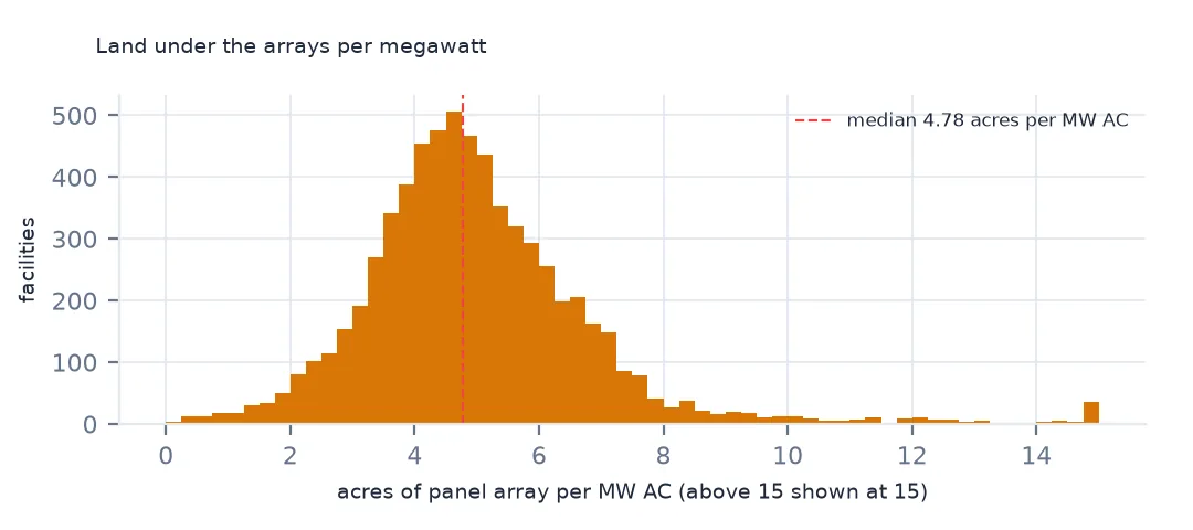
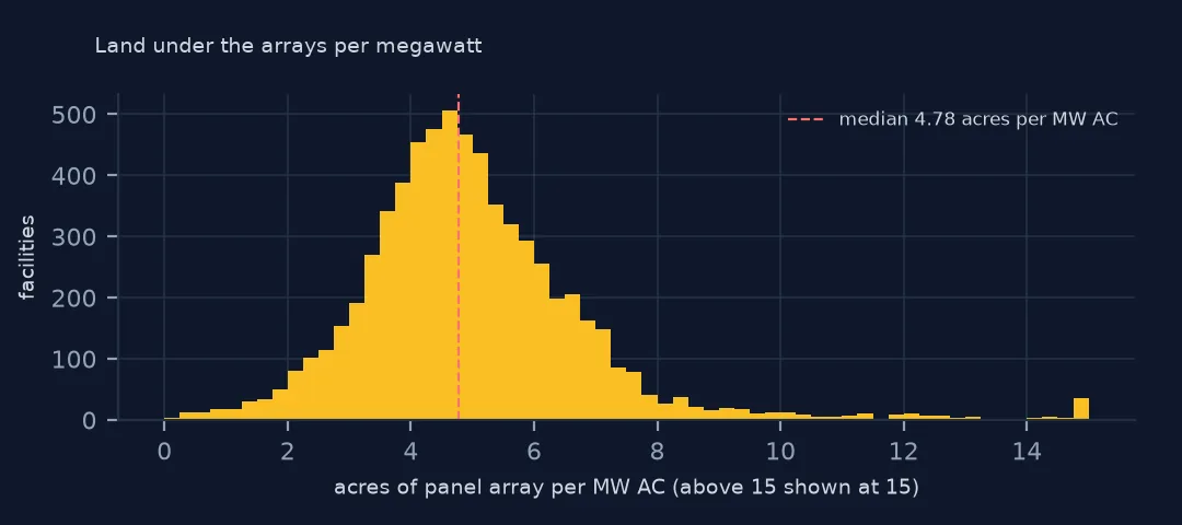
acres of array per MW AC: median 4.78; middle half 3.90-5.86
Across all facilities, the arrays hold 57.1 MW DC per km², and the median facility 66.6. In planners' units, the median facility uses 4.78 acres of array per MW AC, and the middle half 3.90 to 5.86. The larger figures that circulate in planning debates count the fenced area around the arrays, with roads and gaps, which this database does not draw.
Mounting, year and the outliers
1. By mounting
g = pv.groupby("p_axis").agg(n=("case_id", "size"), mw=("p_cap_dc", "sum"), km2=("p_area", lambda a: a.sum() / 1e6))
g["mw_per_km2"] = g.mw / g.km2
print(g[g.n >= 20].round(1).to_string())
n mw km2 mw_per_km2
p_axis
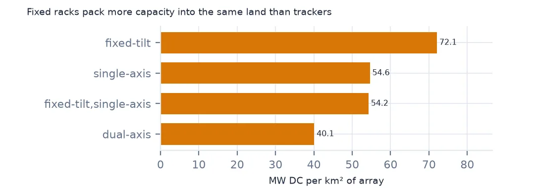
dual-axis 49 798.6 19.9 40.1
fixed-tilt 3109 29222.6 405.4 72.1
fixed-tilt,single-axis 21 366.9 6.8 54.2
single-axis 3146 119029.4 2180.8 54.6
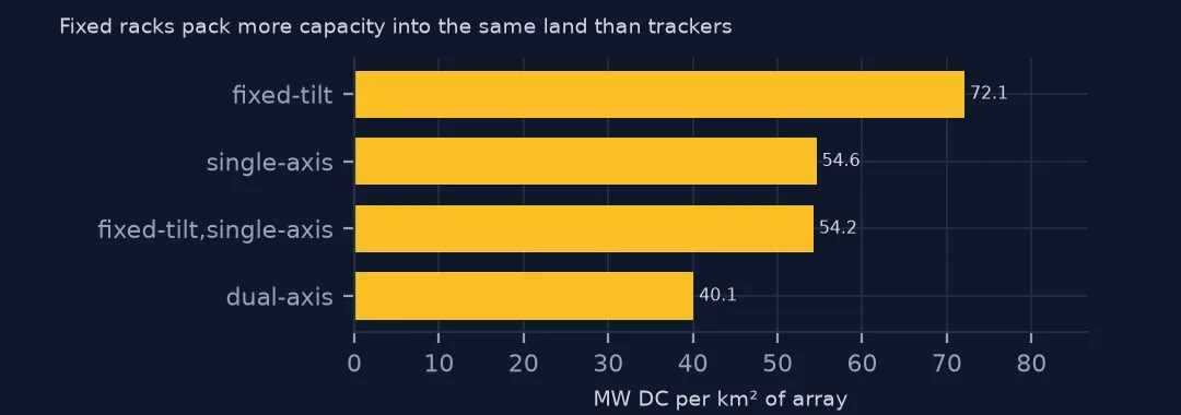
Fixed-tilt arrays are the densest, 72.1 MW DC per km² of array, and single-axis trackers hold 54.6. Trackers turn to follow the sun and must be spaced so their rows do not shade each other when tilted at morning and evening; fixed rows can sit closer. Trackers produce more energy per megawatt, so per unit of energy the gap is smaller than per unit of capacity.
2. By year
y = pv[pv.p_year >= 2010].groupby("p_year").agg(mw=("p_cap_dc", "sum"), km2=("p_area", lambda a: a.sum() / 1e6))
print((y.mw / y.km2).round(1).to_string())
p_year
2010 44.5
2011 57.4
2012 57.3
2013 55.1
2014 55.6
2015 59.0
2016 54.8
2017 59.8
2018 63.1
2019 66.1
2020 56.8
2021 61.6
2022 58.4
2023 54.7
2024 55.1
2025 53.8
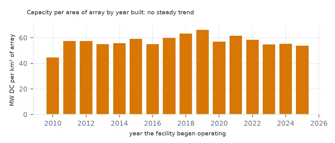
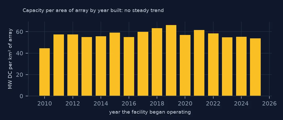
Density by year built changes little: between 54 and 66 MW DC per km² since 2011, with no steady trend. Panels have become more efficient, but the shift to trackers, which need more space, has probably offset the gain.
3. Outliers the database flags
flag = pv[pv.p_zscore.abs() > 3]
print(f"|z| > 3: {len(flag)}; median MW DC per km² among them: {(flag.p_cap_dc / (flag.p_area / 1e6)).median():.0f}")
print(flag.assign(d=(flag.p_cap_dc / (flag.p_area / 1e6)).round(0)).nlargest(4, "d")[["p_name", "p_state", "p_sys_type", "p_cap_dc", "p_area", "d"]].to_string(index=False))
|z| > 3: 60; median MW DC per km² among them: 444
p_name p_state p_sys_type p_cap_dc p_area d
Elm Street MA rooftop 3.7 869 4258.0
Maverick Solar 7, LLC CA ground 179.0 62529 2863.0
Howell CSG NY ground 3.0 2381 1260.0
Halifax Solar MA rooftop 3.1 2799 1108.0
The database flags its own doubtful records with p_zscore, the z-score of capacity per area. 60 facilities lie more than three standard deviations out, with a median of 444 MW DC per km², several times any real array. The top of the list is a rooftop in Massachusetts with 3.7 MW on 869 m², and Maverick Solar 7 in California, 179 MW on 62,529 m², where the outline evidently covers only part of the plant. Drop or check them before quoting land use.
The land in all US solar arrays
The data used on this page
The US Geological Survey and Lawrence Berkeley National Laboratory's US Large-Scale Solar Photovoltaic Database (USPVDB), version 4.0 of 14 April 2026 (Fujita and others, doi:10.5066/P9IA3TUS), public domain, as GeoJSON with the metadata and changelog from the download. USGS replaces the files at the same address with each version, so version 4.0 was saved on this site on 28 October 2026. Capacities are megawatts, areas square metres of panels and inverters.
from pathlib import Path
import zipfile

import geopandas as gpd
import numpy as np
import pandas as pd
import requests

Path("data").mkdir(exist_ok=True)
# USGS/LBNL US Large-Scale Solar Photovoltaic Database (USPVDB) version 4.0 of April 2026 (doi:10.5066/P9IA3TUS),
# array outlines as GeoJSON, with the Census Bureau's 2024 counties and states. Saved 28 October 2026: each new
# version replaces the files at the same address.
# Live: https://energy.usgs.gov/uspvdb/assets/data/uspvdbGeoJSON.zip
ARCHIVE = "usgs-uspvdb-v4-0-2026-10-28.zip"
if not Path(f"data/{ARCHIVE}").exists():
    Path(f"data/{ARCHIVE}").write_bytes(requests.get(f"https://data.spatialworkflow.io/{ARCHIVE}", timeout=600).content)
Z = zipfile.ZipFile(f"data/{ARCHIVE}")
for f in ["uspvdb_v4_0_20260414.geojson", "cb_2024_us_county_20m.zip", "cb_2024_us_state_20m.zip"]:
    if not Path(f"data/{f}").exists():
        Path(f"data/{f}").write_bytes(Z.read(f))
pv = gpd.read_file("data/uspvdb_v4_0_20260414.geojson")
print(f"USPVDB 4.0: {len(pv):,} solar facilities, {pv.p_cap_ac.sum():,.0f} MW AC")
USPVDB 4.0: 6,611 solar facilities, 131,574 MW AC
Example 1: the land in all US solar arrays
km2 = pv.p_area.sum() / 1e6
print(f"array area: {km2:,.0f} km² ({km2 * 247.105:,.0f} acres) for {pv.p_cap_ac.sum():,.0f} MW AC")
big = pv[pv.p_cap_ac >= 100]
print(f"facilities of 100 MW AC or more: {len(big)}, {big.p_area.sum() / pv.p_area.sum():.1%} of the array area")
array area: 2,852 km² (704,769 acres) for 131,574 MW AC
facilities of 100 MW AC or more: 406, 58.3% of the array area
Together, the arrays cover 2,852 km², 704,769 acres, for 131,574 MW AC, an area a little larger than Rhode Island's land. The 406 facilities of 100 MW AC or more account for 58.3% of it.
Internal links
- Trackers and fixed tilt — where each mounting is used
- Solar farm areas — computing the area yourself
- AC and DC capacity — which megawatts to divide by
- Solar on landfills — land that was already used