
Fixing Solar Capacity Totals That Mix AC and DC Megawatts
On this page
Problem statement
A solar farm has two capacities. The DC rating is the sum of its panels' nameplate power; the AC rating is what its inverters can deliver to the grid, and it is lower, because plants are built with more panels than inverter capacity. EIA's statistics, utility reports and most news use AC; developers and panel makers often quote DC. The USPVDB carries both, p_cap_ac and p_cap_dc, and a total that takes one figure from one source and another from another can be off by a fifth. This page measures the ratio between them, finds the records where it cannot be right, and shows how large a mixed total goes wrong.
Quick answer
Sum each column and look at the DC/AC ratio, the inverter loading ratio, for every facility:
print(f"MW AC: {pv.p_cap_ac.sum():,.0f}; MW DC: {pv.p_cap_dc.sum():,.0f}; difference: {pv.p_cap_dc.sum() - pv.p_cap_ac.sum():,.0f} MW")
ilr = pv.p_cap_dc / pv.p_cap_ac
print(ilr.describe(percentiles=[0.05, 0.5, 0.95]).round(2).to_string())
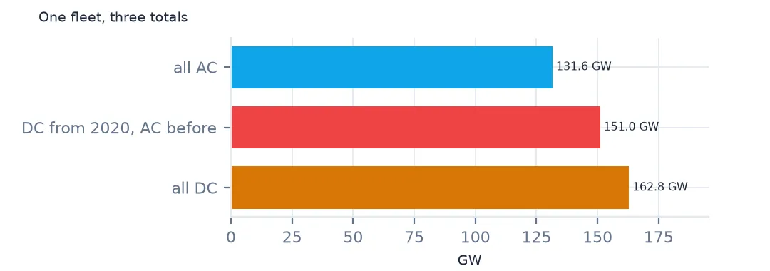
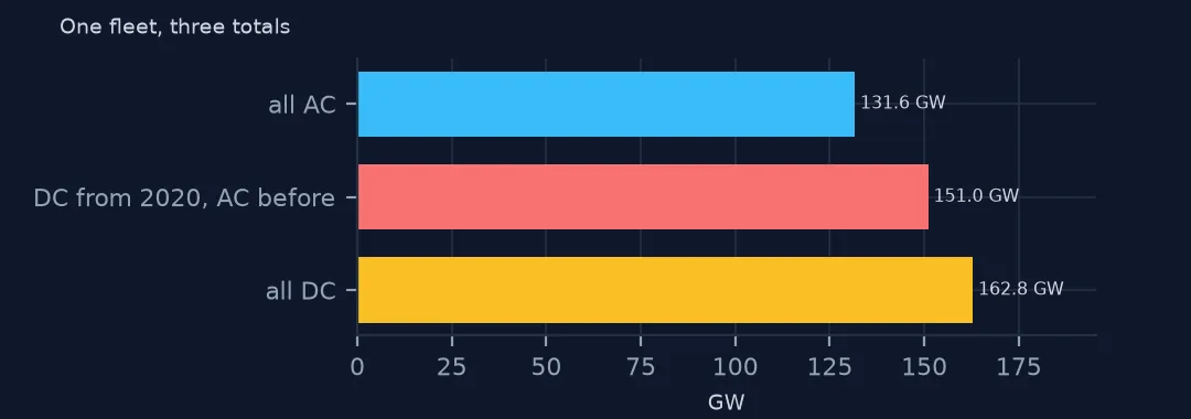
MW AC: 131,574; MW DC: 162,802; difference: 31,229 MW
count 6611.00
mean 1.29
std 0.23
min 0.01
5% 1.00
50% 1.30
95% 1.50
max 7.00
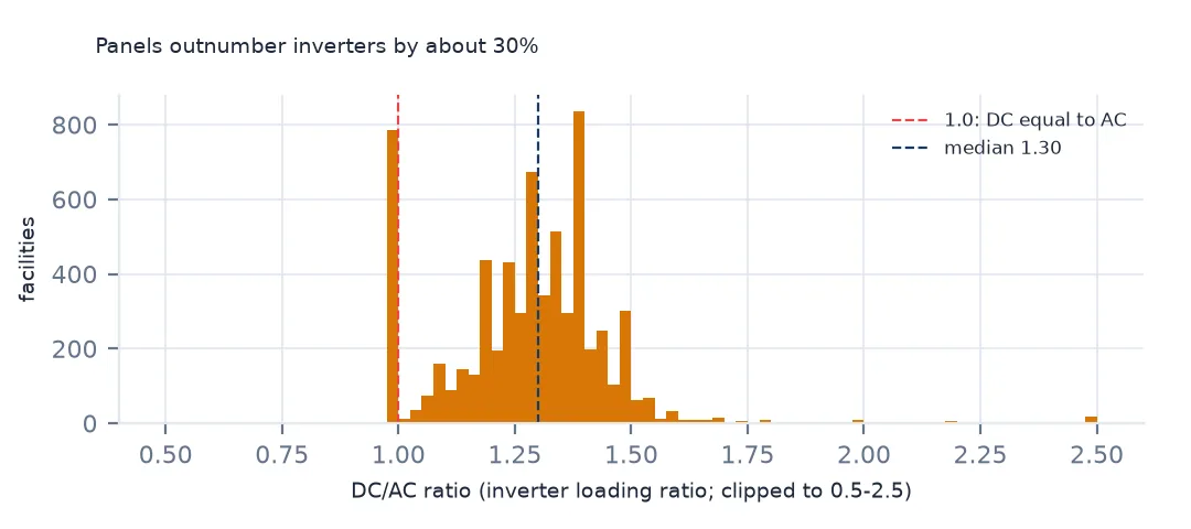
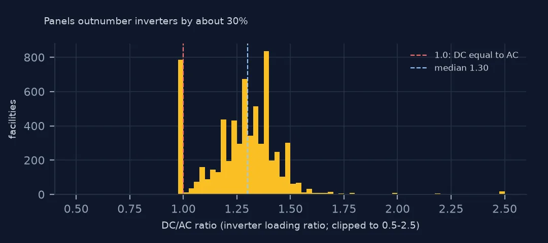
The facilities hold 131,574 MW AC and 162,802 MW DC, a difference of 31,229 MW. The DC/AC ratio, called the inverter loading ratio, has a median of 1.30, and 90% of facilities lie between 1.00 and 1.50. The extremes, 0.01 and 7.00, are errors.
The ratio, its errors and the cost of mixing
1. What the ratio is
print(pv.assign(ilr=ilr).groupby("p_axis").ilr.median().round(2).to_string())
print(pv.assign(ilr=ilr)[pv.p_year >= 2012].groupby("p_year").ilr.median().round(2).to_string())
y25 = pv[pv.p_year == 2025]
print(f"2025 facilities: DC equal to AC {(y25.p_cap_dc == y25.p_cap_ac).mean():.0%}; no mounting reported {y25.p_axis.isna().mean():.0%}")
p_axis
dual-axis 1.22
dual-axis,fixed-tilt,single-axis 1.11
fixed-tilt 1.30
fixed-tilt,single-axis 1.20
single-axis 1.30
p_year
2012 1.21
2013 1.25
2014 1.27
2015 1.29
2016 1.31
2017 1.33
2018 1.33
2019 1.35
2020 1.35
2021 1.35
2022 1.32
2023 1.29
2024 1.25
2025 1.00
2025 facilities: DC equal to AC 96%; no mounting reported 100%
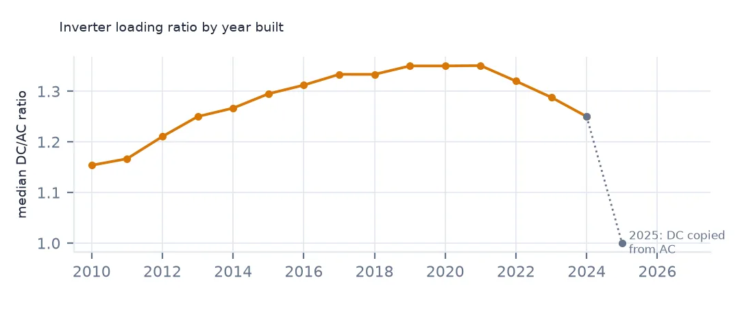
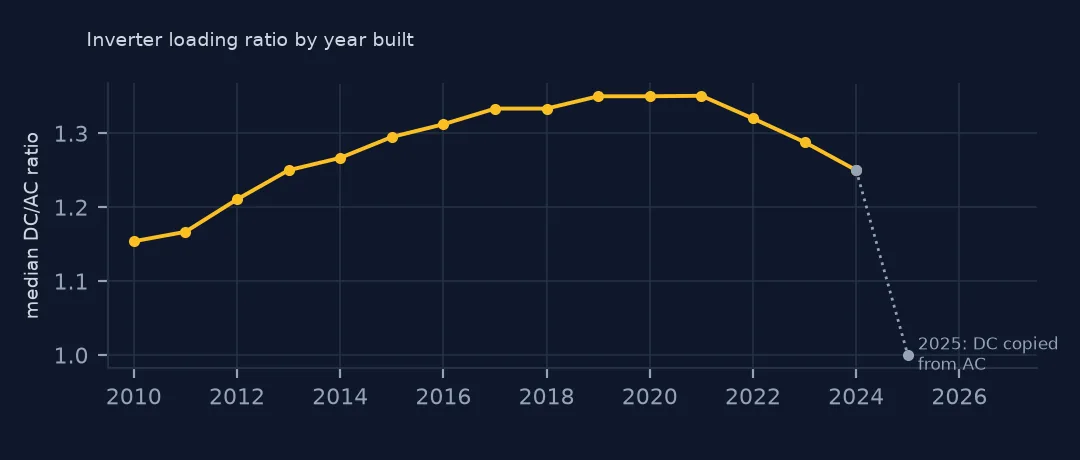
The ratio is about 1.30 for both fixed-tilt and single-axis plants. By year it rose from 1.21 in 2012 to 1.35 in 2019–2021, as cheaper panels made it worth oversizing the arrays, and has fallen to 1.25 for 2024 plants. The 2025 value of 1.00 is not real: 96% of 2025 facilities have DC equal to AC, and none reports a mounting. Until EIA's detail arrives, the newest plants' DC column is a copy of AC.
2. Ratios that cannot be right
bad = pv[(ilr < 1) | (ilr > 2)]
print(f"DC below AC: {(ilr < 1).sum()}; DC more than twice AC: {(ilr > 2).sum()}")
print(bad.assign(ilr=ilr.round(3)).sort_values("ilr").iloc[[0, 1, -2, -1]][["p_name", "p_state", "p_cap_ac", "p_cap_dc", "ilr"]].to_string(index=False))
DC below AC: 17; DC more than twice AC: 41
p_name p_state p_cap_ac p_cap_dc ilr
Texas Solar Nova 1 TX 252.0 1.8 0.007
RE McKenzie 1, LLC CA 30.0 6.3 0.210
Stafford St Solar 3 (CSG) MA 1.0 6.9 6.900
Bayville Central Facility NJ 0.2 1.4 7.000
17 facilities have less DC than AC, which no real plant can, and 41 have more than twice as much. Texas Solar Nova 1 is listed with 252.0 MW AC and 1.8 MW DC, a ratio of 0.007, clearly a typing error in one column; Bayville Central Facility in New Jersey has 0.2 MW AC against 1.4 MW DC. Check these outliers against EIA's own tables before using either column for them.
3. Mixing the two
eia_style = pv.p_cap_ac.sum()
mixed = np.where(pv.p_year >= 2020, pv.p_cap_dc, pv.p_cap_ac).sum()
print(f"all AC: {eia_style:,.0f} MW; DC for 2020 and later, AC before: {mixed:,.0f} MW ({mixed / eia_style - 1:+.1%})")
all AC: 131,574 MW; DC for 2020 and later, AC before: 150,995 MW (+14.8%)
Mixing the columns is easy to do by accident, for instance by taking recent plants from a developer list in DC and older ones from EIA in AC. Using DC for facilities from 2020 on and AC before gives 150,995 MW instead of 131,574, 14.8% too high. Choose one column for every total, and say which.
Capacity density in consistent units
The data used on this page
The US Geological Survey and Lawrence Berkeley National Laboratory's US Large-Scale Solar Photovoltaic Database (USPVDB), version 4.0 of 14 April 2026 (Fujita and others, doi:10.5066/P9IA3TUS), public domain, as GeoJSON with the metadata and changelog from the download. USGS replaces the files at the same address with each version, so version 4.0 was saved on this site on 28 October 2026. Capacities are megawatts, areas square metres of panels and inverters.
from pathlib import Path
import zipfile

import geopandas as gpd
import numpy as np
import pandas as pd
import requests

Path("data").mkdir(exist_ok=True)
# USGS/LBNL US Large-Scale Solar Photovoltaic Database (USPVDB) version 4.0 of April 2026 (doi:10.5066/P9IA3TUS),
# array outlines as GeoJSON, with the Census Bureau's 2024 counties and states. Saved 28 October 2026: each new
# version replaces the files at the same address.
# Live: https://energy.usgs.gov/uspvdb/assets/data/uspvdbGeoJSON.zip
ARCHIVE = "usgs-uspvdb-v4-0-2026-10-28.zip"
if not Path(f"data/{ARCHIVE}").exists():
    Path(f"data/{ARCHIVE}").write_bytes(requests.get(f"https://data.spatialworkflow.io/{ARCHIVE}", timeout=600).content)
Z = zipfile.ZipFile(f"data/{ARCHIVE}")
for f in ["uspvdb_v4_0_20260414.geojson", "cb_2024_us_county_20m.zip", "cb_2024_us_state_20m.zip"]:
    if not Path(f"data/{f}").exists():
        Path(f"data/{f}").write_bytes(Z.read(f))
pv = gpd.read_file("data/uspvdb_v4_0_20260414.geojson")
print(f"USPVDB 4.0: {len(pv):,} solar facilities, {pv.p_cap_ac.sum():,.0f} MW AC")
USPVDB 4.0: 6,611 solar facilities, 131,574 MW AC
Example 1: capacity density in consistent units
for col in ["p_cap_ac", "p_cap_dc"]:
    print(col, f"{pv[col].sum() / (pv.p_area.sum() / 1e6):.1f} MW per km² of array")
p_cap_ac 46.1 MW per km² of array
p_cap_dc 57.1 MW per km² of array
The same choice changes every density. Per square kilometre of array, the facilities hold 46.1 MW AC or 57.1 MW DC. Land-use figures in the literature are quoted both ways, so compare like with like.
Internal links
- Reading the database — both columns in context
- Solar farm land use — the density figures this page corrects
- Solar growth by year — capacity by year, in AC
- Power plants from EIA-860 — the source of both columns