
How to Read the US Large-Scale Solar Photovoltaic Database in Python
On this page
Problem statement
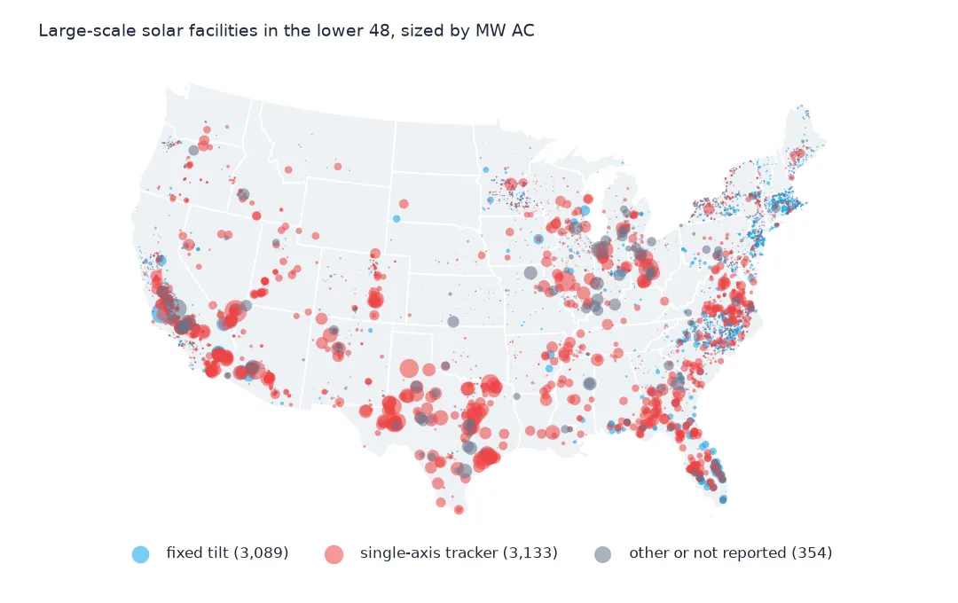
The US Large-Scale Solar Photovoltaic Database (USPVDB) maps every solar facility in the country with a capacity of a megawatt or more: 6,611 of them in version 4.0, from community solar fields in Massachusetts to Gemini Solar in the Nevada desert. Each record is an outline of the panel arrays, digitised from aerial imagery, joined to the plant's entry in the Energy Information Administration's Form 860, with its AC and DC capacity, year, mounting, panel type and land use. This page reads the GeoJSON, checks the ids, capacities, points and dates, and shows what the table holds.
Quick answer
Read the GeoJSON with GeoPandas; each row is one facility with its outline:
print(pv[["case_id", "p_name", "p_state", "p_county", "p_year", "p_cap_ac", "p_cap_dc", "p_area", "p_axis"]].head(3).to_string(index=False))
print(pv.crs, pv.geom_type.value_counts().to_dict())
case_id p_name p_state p_county p_year p_cap_ac p_cap_dc p_area p_axis
400011 Mustang OK Canadian 2015 2.5 3.0 50723 single-axis
407013 Comfort CSG NY Erie 2024 4.0 5.5 77051 single-axis
404351 Viking Solar (CSG) IL Macoupin 2021 2.0 3.0 56943 single-axis
EPSG:4326 {'Polygon': 3529, 'MultiPolygon': 3082}
The first rows are small: Mustang, a 2.5 MW AC array in Canadian County, Oklahoma, and two community solar fields in New York and Illinois. The geometries are in EPSG:4326, 3,529 single polygons and 3,082 multipolygons. p_area is the array area in square metres, already computed in an equal-area projection.
The records, the capacities and the dates
1. One record per facility
print(f"case_id unique: {pv.case_id.is_unique}; eia_id unique: {pv.eia_id.is_unique}; states: {pv.p_state.nunique()}")
print(pv.multi_poly.value_counts().to_dict())
print(f"polygons in the multi-part records: {pv[pv.multi_poly == 'multi'].geometry.apply(lambda g: len(getattr(g, 'geoms', [g]))).describe()[['mean', 'max']].round(1).to_dict()}")
case_id unique: True; eia_id unique: True; states: 50
{'single': 3529, 'multi': 3082}
polygons in the multi-part records: {'mean': 5.4, 'max': 126.0}
case_id is the database's own stable id and eia_id the EIA plant code; both are unique, so each EIA plant appears once. The 6,611 facilities carry 50 different state codes. 3,082 records are multi-part, a plant whose arrays are separate fields; they average 5.4 parts, and one has 126.
2. Two capacities
print(f"MW AC: {pv.p_cap_ac.sum():,.0f}; MW DC: {pv.p_cap_dc.sum():,.0f}; DC/AC: {pv.p_cap_dc.sum() / pv.p_cap_ac.sum():.3f}")
print(pv.p_cap_ac.describe(percentiles=[0.25, 0.5, 0.75, 0.99]).round(1).to_string())
MW AC: 131,574; MW DC: 162,802; DC/AC: 1.237
count 6611.0
mean 19.9
std 50.2
min 0.2
25% 1.8
50% 3.2
75% 7.0
99% 250.0
max 690.0
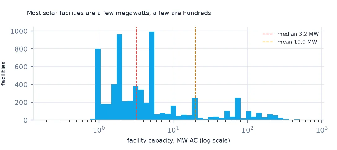
The table has two capacities: 131,574 MW AC, what the inverters deliver to the grid, and 162,802 MW DC, the panels' rating, 1.237 times as much. Sizes are very uneven. The median facility is 3.2 MW AC, three quarters are 7.0 MW or smaller, and the largest is 690 MW; the mean of 19.9 MW describes few facilities. Sum one column only; the AC and DC page shows how far mixing them goes wrong.
3. The point and the outline
pts = gpd.GeoSeries(gpd.points_from_xy(pv.xlong, pv.ylat), crs=4269).to_crs(pv.crs)
inside = pts.within(pv.geometry.reset_index(drop=True))
print(f"representative point inside its outline: {inside.mean():.1%}; outside: {(~inside).sum()}")
print(pv[~inside.values].multi_poly.value_counts().to_dict())
representative point inside its outline: 99.1%; outside: 61
{'multi': 52, 'single': 9}
ylat and xlong are a representative point for each facility, in NAD83. 99.1% lie inside their own outline. Of the 61 that don't, 52 belong to multi-part facilities, where the point is placed between separate fields. For a dot map the points are fine; for anything about land, use the outline.
4. Dates
print(f"operating since: {pv.p_year.min()} to {pv.p_year.max()}")
img = pd.to_datetime(pv.p_img_date.astype(str), format="%Y%m%d", errors="coerce")
print(f"image dates that are not dates: {img.isna().sum()} {pv.loc[img.isna(), 'p_img_date'].tolist()}")
print(f"imagery: {img.min():%Y-%m-%d} to {img.max():%Y-%m-%d}; imaged before the year it began operating: {(img.dt.year < pv.p_year).sum()}")
operating since: 1985 to 2025
image dates that are not dates: 1 [20240231]
imagery: 2009-04-17 to 2026-02-08; imaged before the year it began operating: 136
The facilities began operating between 1985 and 2025. Each outline was checked against an aerial image, dated in p_img_date as an integer, and one of those dates, 20240231, is 31 February: parse with errors="coerce" or the whole column fails. The images run from 2009 to February 2026, and 136 facilities were imaged before the year they began operating, so their outline shows the site under construction.
Capacity by state and by mounting place
The data used on this page
The US Geological Survey and Lawrence Berkeley National Laboratory's US Large-Scale Solar Photovoltaic Database (USPVDB), version 4.0 of 14 April 2026 (Fujita and others, doi:10.5066/P9IA3TUS), public domain, as GeoJSON with the metadata and changelog from the download. USGS replaces the files at the same address with each version, so version 4.0 was saved on this site on 28 October 2026. Capacities are megawatts, areas square metres of panels and inverters.
from pathlib import Path
import zipfile

import geopandas as gpd
import numpy as np
import pandas as pd
import requests

Path("data").mkdir(exist_ok=True)
# USGS/LBNL US Large-Scale Solar Photovoltaic Database (USPVDB) version 4.0 of April 2026 (doi:10.5066/P9IA3TUS),
# array outlines as GeoJSON, with the Census Bureau's 2024 counties and states. Saved 28 October 2026: each new
# version replaces the files at the same address.
# Live: https://energy.usgs.gov/uspvdb/assets/data/uspvdbGeoJSON.zip
ARCHIVE = "usgs-uspvdb-v4-0-2026-10-28.zip"
if not Path(f"data/{ARCHIVE}").exists():
    Path(f"data/{ARCHIVE}").write_bytes(requests.get(f"https://data.spatialworkflow.io/{ARCHIVE}", timeout=600).content)
Z = zipfile.ZipFile(f"data/{ARCHIVE}")
for f in ["uspvdb_v4_0_20260414.geojson", "cb_2024_us_county_20m.zip", "cb_2024_us_state_20m.zip"]:
    if not Path(f"data/{f}").exists():
        Path(f"data/{f}").write_bytes(Z.read(f))
pv = gpd.read_file("data/uspvdb_v4_0_20260414.geojson")
print(f"USPVDB 4.0: {len(pv):,} solar facilities, {pv.p_cap_ac.sum():,.0f} MW AC")
USPVDB 4.0: 6,611 solar facilities, 131,574 MW AC
Example 1: capacity by state
st = pv.groupby("p_state").agg(facilities=("case_id", "size"), mw_ac=("p_cap_ac", "sum")).sort_values("mw_ac", ascending=False)
print(st.head(8).round(0).astype(int).to_string())
print(f"top 5 states' share of capacity: {st.mw_ac.head(5).sum() / st.mw_ac.sum():.1%}")
facilities mw_ac
p_state
TX 187 23033
CA 893 22881
FL 202 11622
NC 760 6697
AZ 110 5488
GA 152 5364
NV 66 4759
VA 124 4710
top 5 states' share of capacity: 53.0%
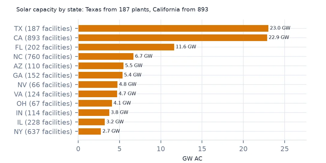
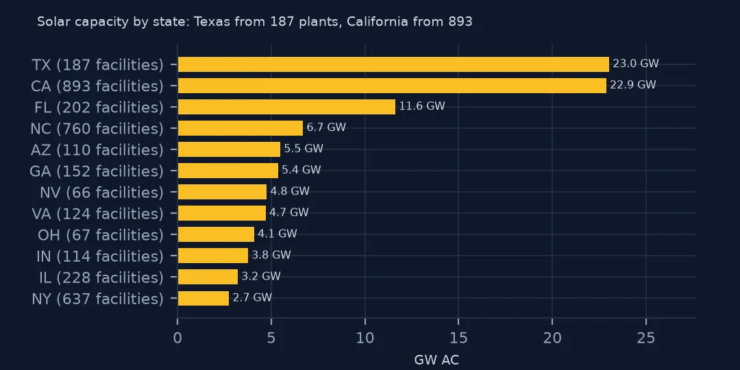
Texas and California lead with 23,033 and 22,881 MW AC, but California has 893 facilities against Texas's 187: Texas builds fewer, much larger plants. Florida, North Carolina, Arizona, Georgia, Nevada and Virginia follow, and the five largest states hold 53.0% of the capacity. North Carolina's 760 facilities are small ones: 6,697 MW between them.
Example 2: where the panels sit
print(pv.groupby("p_sys_type").agg(facilities=("case_id", "size"), mw_ac=("p_cap_ac", "sum"), median_mw=("p_cap_ac", "median")).sort_values("facilities", ascending=False).round(1).to_string()) facilities mw_ac median_mw
p_sys_type
ground 5976 130336.2 4.0
rooftop 407 782.7 1.5
canopy 148 293.4 1.5
canopy,rooftop 62 120.1 1.5
canopy,ground 7 15.0 1.5
canopy,ground,rooftop 5 15.2 3.7
ground,rooftop 4 6.8 1.8
floating 2 4.1 2.0
Ground-mounted systems are 5,976 facilities and 130,336 MW AC, nearly all the capacity. 407 rooftop and 148 parking-canopy systems are mostly small, with medians of 1.5 MW, and two floating arrays add 4.1 MW. The database's p_sys_type comes from the imagery, so it describes what the panels sit on, not what EIA reports.
Internal links
- The database explained — what it counts and leaves out, and getting the data without code
- AC and DC capacity — the two megawatt columns
- Solar capacity by county — the facilities on a map
- Solar farm areas — computing area from the outlines