
How to Map Solar Farm Capacity by County
On this page
Problem statement
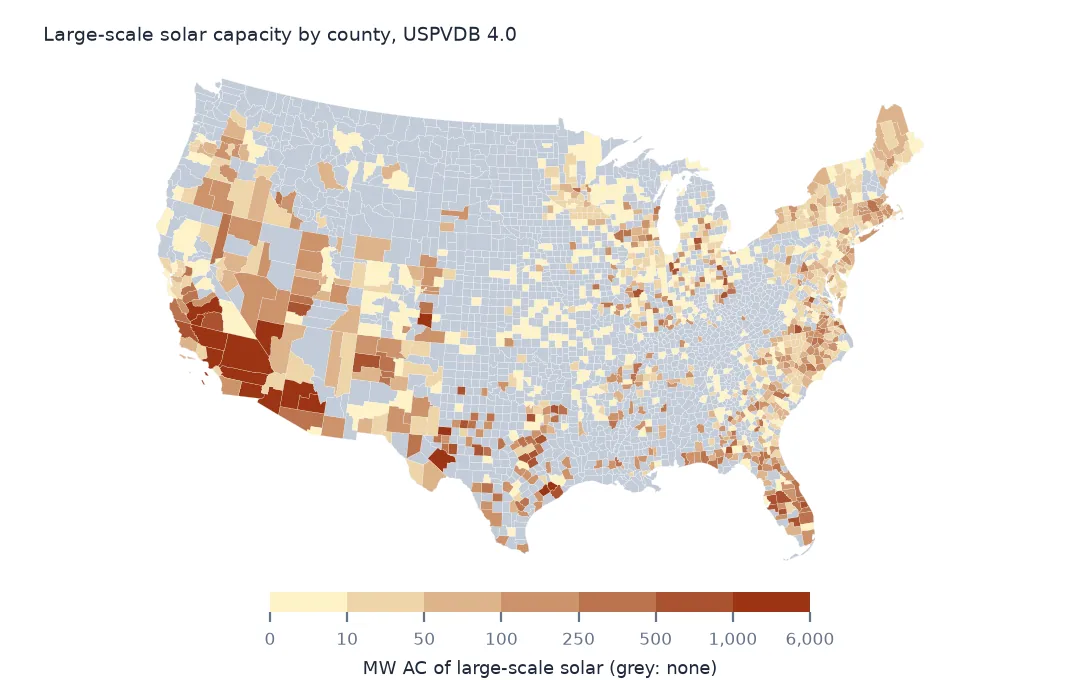
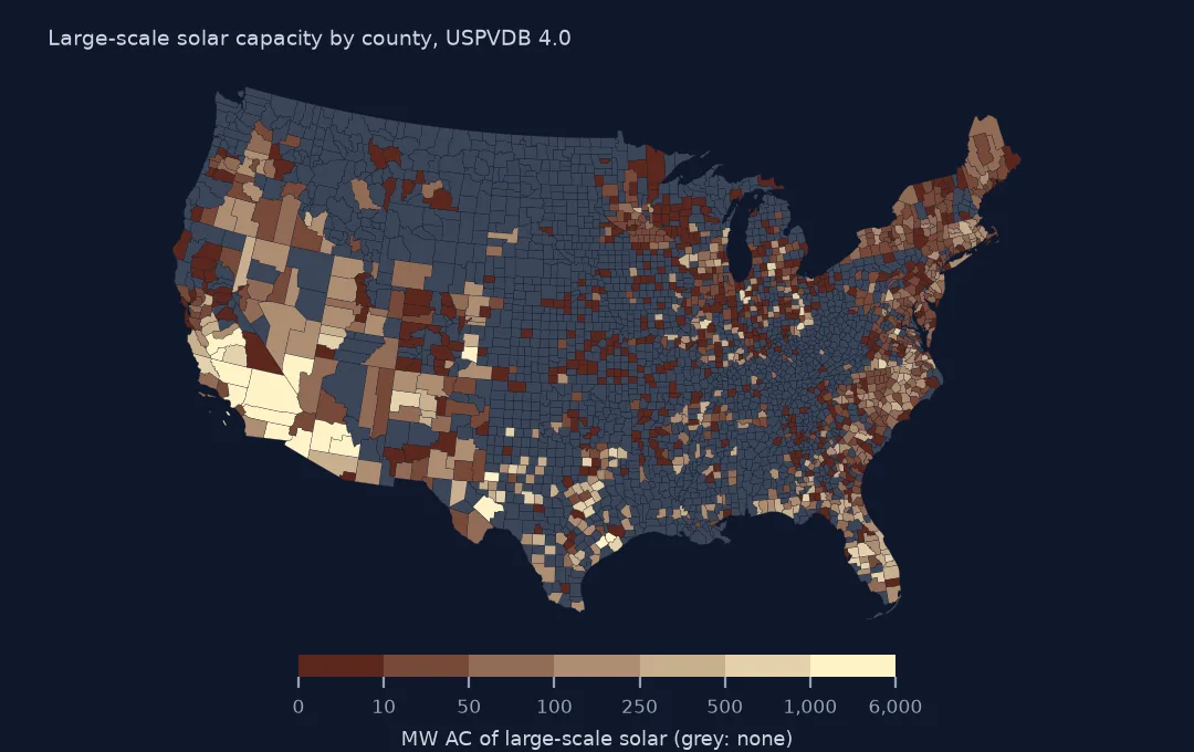
Utility-scale solar is concentrated in a small number of counties, and a county map is the clearest way to show where. The USPVDB gives each facility a county name, but names repeat across states and Connecticut's counties no longer exist in the Census Bureau's boundaries, so the reliable join is spatial: each facility's representative point into the county polygons. This page joins the 6,611 facilities to counties, checks the file's county names, measures how concentrated the capacity is, and ranks counties by capacity per area.
Quick answer
Build points from xlong and ylat, join them to the 2024 county boundaries and sum capacity per county:
counties = gpd.read_file("data/cb_2024_us_county_20m.zip")
pts = gpd.GeoDataFrame(pv.drop(columns="geometry"), geometry=gpd.points_from_xy(pv.xlong, pv.ylat), crs=4269).to_crs(counties.crs)
j = gpd.sjoin(pts, counties[["GEOID", "NAMELSAD", "STUSPS", "geometry"]], how="left", predicate="within")
per = j.groupby("GEOID").agg(facilities=("case_id", "size"), mw_ac=("p_cap_ac", "sum"))
print(f"counties with a facility: {len(per):,} of {len(counties):,}; points in no county: {j.GEOID.isna().sum()}")
print(per.join(counties.set_index("GEOID")[["NAMELSAD", "STUSPS"]]).nlargest(6, "mw_ac").round(0).to_string())
counties with a facility: 1,237 of 3,222; points in no county: 1
facilities mw_ac NAMELSAD STUSPS
GEOID
06029 140 5838.0 Kern County CA
06065 64 4358.0 Riverside County CA
32003 42 3695.0 Clark County NV
04013 37 2461.0 Maricopa County AZ
06025 36 2106.0 Imperial County CA
48371 12 2073.0 Pecos County TX
1,237 of the 3,222 counties have at least one large solar facility; one point falls in no county. Kern County, California, leads with 140 facilities and 5,838 MW AC, then Riverside County with 4,358 MW and Clark County, Nevada, with 3,695. Pecos County, Texas, is sixth with 2,073 MW from only 12 facilities.
The join and what it shows
1. The county name in the file
name = j.NAMELSAD.str.replace(r" (County|Parish|Borough|Census Area|city|City and Borough|Municipality)$", "", regex=True)
print(f"p_county equals the joined county name: {(j.p_county == name).mean():.1%}")
print(j.loc[j.p_county != name, ["p_county", "NAMELSAD", "STUSPS"]].drop_duplicates().head(5).to_string(index=False))
p_county equals the joined county name: 97.5%
p_county NAMELSAD STUSPS
Hartford Capitol Planning Region CT
Litchfield Northwest Hills Planning Region CT
Jackson Calhoun County MI
New Haven Naugatuck Valley Planning Region CT
Geary Riley County KS
The file's p_county matches the joined county's name for 97.5% of facilities. Most mismatches are Connecticut, where the file uses the old county names, Hartford, Litchfield, New Haven, and the 2024 boundaries use the planning regions that replaced them. The rest are facilities near a county line, such as one listed in Jackson County, Michigan, whose point lies in Calhoun County. Join on geometry, not on names.
2. How concentrated
s = per.mw_ac.sort_values(ascending=False)
print(f"largest 1% of solar counties hold {s.head(int(len(s) * 0.01)).sum() / s.sum():.1%} of capacity; largest 10%: {s.head(int(len(s) * 0.1)).sum() / s.sum():.1%}")
print(f"counties with one facility: {(per.facilities == 1).sum()}")
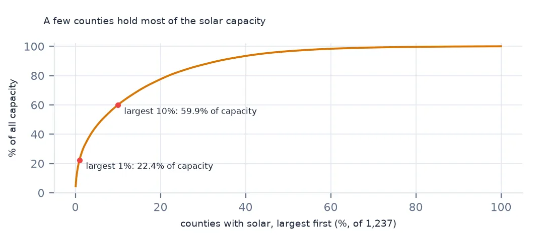
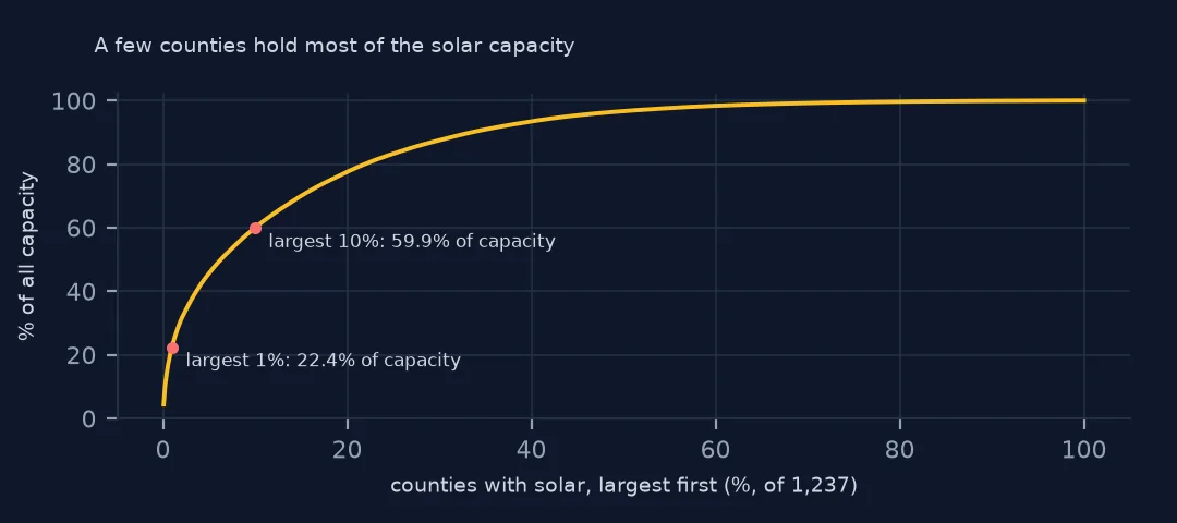
largest 1% of solar counties hold 22.4% of capacity; largest 10%: 59.9%
counties with one facility: 494
Capacity is concentrated. The largest 1% of solar counties hold 22.4% of all capacity, and the largest 10% hold 59.9%. At the other end, 494 counties have a single facility, mostly a community solar field of a few megawatts.
3. Per area of county
c = counties.merge(per, left_on="GEOID", right_index=True, how="left")
c["mw_per_1000_km2"] = c.mw_ac / (c.to_crs(5070).area / 1e9)
print(c.nlargest(5, "mw_per_1000_km2")[["NAMELSAD", "STUSPS", "mw_ac", "mw_per_1000_km2"]].round(1).to_string(index=False))
NAMELSAD STUSPS mw_ac mw_per_1000_km2
Madison County OH 957.2 801.1
Surry County VA 395.9 510.0
Starke County IN 400.0 492.0
Jasper County IN 705.0 490.7
Jeff Davis County GA 413.5 486.5
Per 1,000 km² of county, the densest solar counties are not in the desert: Madison County, Ohio, with 801 MW per 1,000 km², Surry County, Virginia, Starke and Jasper Counties, Indiana, and Jeff Davis County, Georgia. Each holds one or two very large plants in a small county. Kern County's 5,838 MW is spread over a county the size of a small state.
Each state's solar counties
The data used on this page
The US Geological Survey and Lawrence Berkeley National Laboratory's US Large-Scale Solar Photovoltaic Database (USPVDB), version 4.0 of 14 April 2026 (Fujita and others, doi:10.5066/P9IA3TUS), public domain, as GeoJSON with the metadata and changelog from the download. USGS replaces the files at the same address with each version, so version 4.0 was saved on this site on 28 October 2026. Capacities are megawatts, areas square metres of panels and inverters. County and state boundaries are the Census Bureau's 2024 cartographic boundary files, public domain.
from pathlib import Path
import zipfile

import geopandas as gpd
import numpy as np
import pandas as pd
import requests

Path("data").mkdir(exist_ok=True)
# USGS/LBNL US Large-Scale Solar Photovoltaic Database (USPVDB) version 4.0 of April 2026 (doi:10.5066/P9IA3TUS),
# array outlines as GeoJSON, with the Census Bureau's 2024 counties and states. Saved 28 October 2026: each new
# version replaces the files at the same address.
# Live: https://energy.usgs.gov/uspvdb/assets/data/uspvdbGeoJSON.zip
ARCHIVE = "usgs-uspvdb-v4-0-2026-10-28.zip"
if not Path(f"data/{ARCHIVE}").exists():
    Path(f"data/{ARCHIVE}").write_bytes(requests.get(f"https://data.spatialworkflow.io/{ARCHIVE}", timeout=600).content)
Z = zipfile.ZipFile(f"data/{ARCHIVE}")
for f in ["uspvdb_v4_0_20260414.geojson", "cb_2024_us_county_20m.zip", "cb_2024_us_state_20m.zip"]:
    if not Path(f"data/{f}").exists():
        Path(f"data/{f}").write_bytes(Z.read(f))
pv = gpd.read_file("data/uspvdb_v4_0_20260414.geojson")
print(f"USPVDB 4.0: {len(pv):,} solar facilities, {pv.p_cap_ac.sum():,.0f} MW AC")
USPVDB 4.0: 6,611 solar facilities, 131,574 MW AC
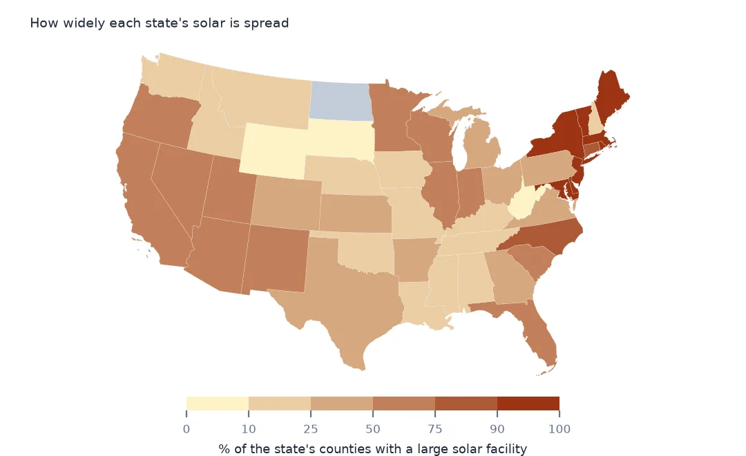
Example 1: the solar share of each state's counties
st = j.groupby("STUSPS").GEOID.nunique().rename("solar_counties").to_frame().join(counties.groupby("STUSPS").size().rename("counties"))
st["share"] = st.solar_counties / st.counties
print(st.sort_values("share", ascending=False).head(6).round(2).to_string())
print(st.sort_values("share").head(4).round(2).to_string())
solar_counties counties share
STUSPS
DC 1 1 1.00
DE 3 3 1.00
NJ 21 21 1.00
RI 5 5 1.00
ME 16 16 1.00
MA 13 14 0.93
solar_counties counties share
STUSPS
SD 3 66 0.05
AK 2 30 0.07
WV 4 55 0.07
WY 2 23 0.09
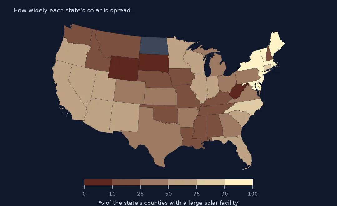
In the smallest eastern states nearly every county has large solar: all of Delaware's, New Jersey's, Rhode Island's and Maine's, and 13 of Massachusetts's 14. South Dakota has large solar in 3 of its 66 counties, West Virginia in 4 of 55 and Wyoming in 2 of 23. Community solar programmes, which put small arrays in many towns, help explain the eastern pattern.
Internal links
- Reading the database — the points and outlines used here
- Wind capacity by county — the same map for wind turbines
- Solar growth by year — which states built when
- Solar farm land use — how much ground a megawatt needs