
How to Compare Single-Axis Tracking and Fixed-Tilt Solar Farms
On this page
Problem statement
Most new American solar farms mount their panels on single-axis trackers, rows that turn from east to west through the day, rather than on fixed racks tilted towards the south. Trackers cost more and need more space, and they produce more energy, especially at low latitudes with clear skies. The USPVDB records each facility's mounting from EIA Form 860, along with tilt and azimuth for fixed arrays. This page counts the two by capacity, follows the shift year by year, tests the latitude pattern, and checks the fixed arrays' tilts.
Quick answer
Group the facilities by mounting, keeping the records with no mounting separate:
pv["mount"] = np.where(pv.p_axis.isna(), "not reported", pv.p_axis.where(pv.p_axis.isin(["single-axis", "fixed-tilt", "dual-axis"]), "mixed"))
t = pv.groupby("mount").agg(facilities=("case_id", "size"), mw_ac=("p_cap_ac", "sum"), median_mw=("p_cap_ac", "median"))
t["share_mw"] = (t.mw_ac / t.mw_ac.sum()).round(3)
print(t.round(1).to_string())
facilities mw_ac median_mw share_mw
mount
dual-axis 49 625.0 2.6 0.0
fixed-tilt 3109 22212.6 2.7 0.2
mixed 23 344.6 3.9 0.0
not reported 284 12926.5 4.6 0.1
single-axis 3146 95464.8 4.8 0.7
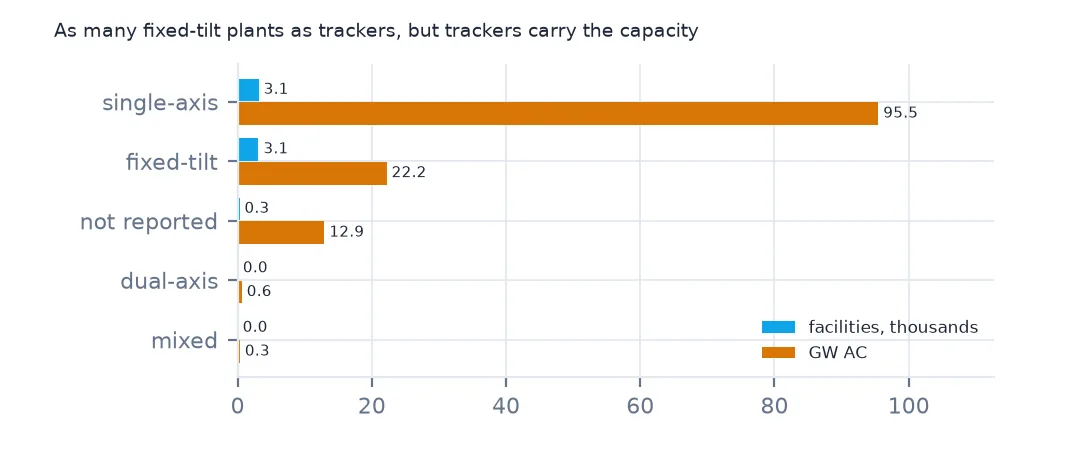
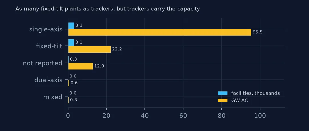
Single-axis trackers carry 95,465 MW AC of the 131,574, almost three quarters, from 3,146 facilities. Fixed-tilt facilities are as numerous, 3,109, but hold only 22,213 MW: their median is 2.7 MW, against 4.8 for trackers. 284 facilities, with 12,927 MW, report no mounting at all, and they are mostly the newest.
Year, latitude and tilt
1. By year built
y = pv[pv.p_year.between(2010, 2025) & (pv.mount != "not reported")]
print(y.groupby("p_year").apply(lambda d: d.loc[d.mount == "single-axis", "p_cap_ac"].sum() / d.p_cap_ac.sum()).map("{:.0%}".format).to_string())
p_year
2010 24%
2011 54%
2012 34%
2013 41%
2014 34%
2015 58%
2016 72%
2017 64%
2018 62%
2019 83%
2020 85%
2021 88%
2022 84%
2023 83%
2024 97%
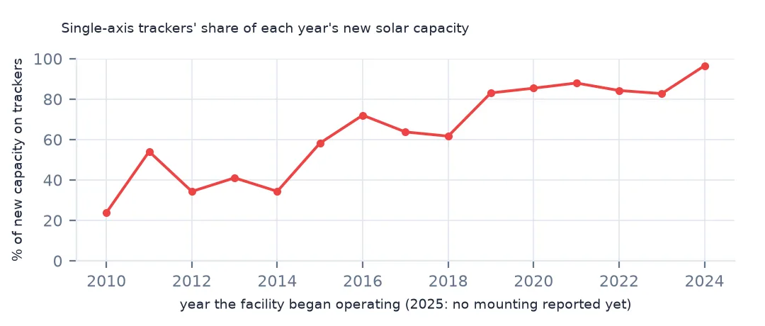
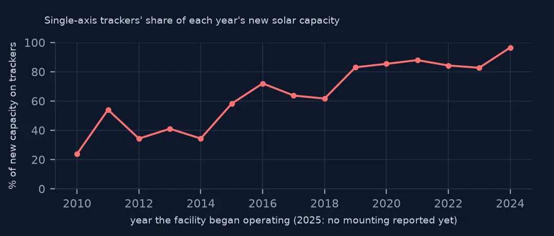
In 2010 trackers carried 24% of the new capacity; from 2016 on they carried most of it, and in 2024 97%. The 2025 facilities are left out because none of them reports a mounting yet: the EIA detail arrives later than the plant.
2. By latitude
band = pd.cut(pv.ylat, [18, 30, 35, 40, 45, 50, 72])
print(pv.groupby(band).apply(lambda d: pd.Series({"facilities": len(d), "single_axis_share": d.loc[d.mount == "single-axis", "p_cap_ac"].sum() / d.p_cap_ac.sum()})).round(2).to_string())
facilities single_axis_share
ylat
(18, 30] 246.0 0.69
(30, 35] 1254.0 0.82
(35, 40] 2047.0 0.71
(40, 45] 2720.0 0.56
(45, 50] 342.0 0.66
(50, 72] 2.0 0.22
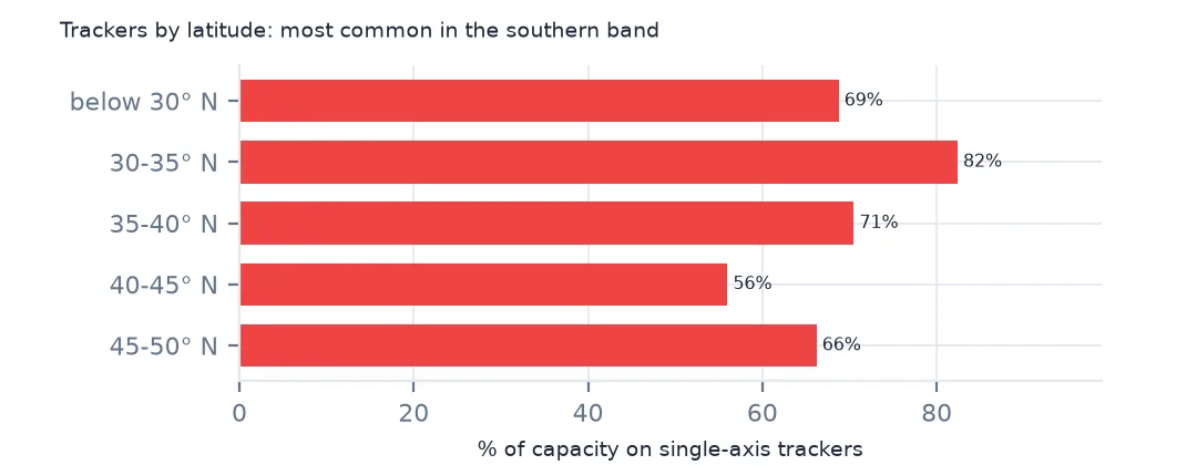
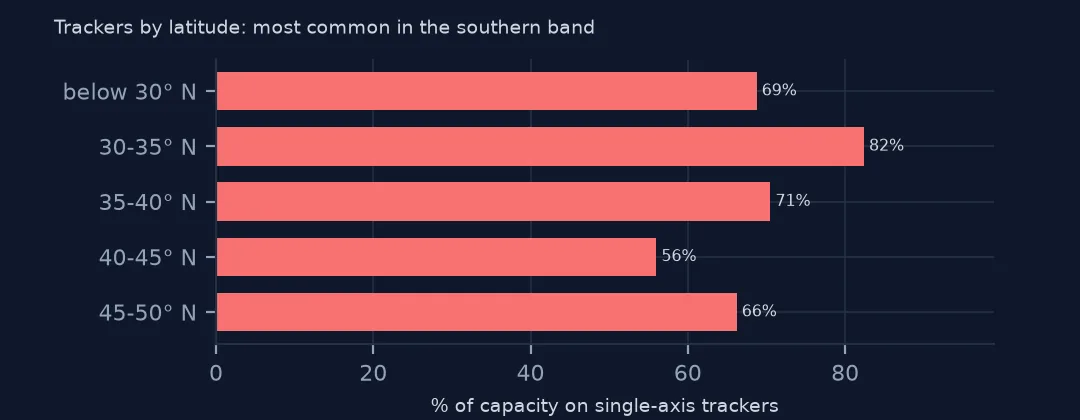
By latitude band, trackers carry 82% of the capacity between 30° and 35° N, the band of Texas, Arizona and southern California, and 56% between 40° and 45° N, where winter sun is low and the fixed share is highest. The tropics and Hawaii, below 30°, are at 69%. The pattern is real but loose: a tracker's gain is largest under clear skies, and plenty of northern plants use them too.
3. Tilt and azimuth of the fixed arrays
f = pv[pv.mount == "fixed-tilt"]
print(f"fixed-tilt with a tilt: {f.p_tilt.notna().sum()}; median tilt {f.p_tilt.median():.0f} degrees; azimuth 180 (due south): {(f.p_azimuth == 180).mean():.1%}")
print(f"correlation of tilt with latitude: {f[['p_tilt', 'ylat']].corr().iloc[0, 1]:.2f}")
fixed-tilt with a tilt: 3066; median tilt 20 degrees; azimuth 180 (due south): 75.2%
correlation of tilt with latitude: 0.19
3,066 fixed-tilt facilities report a tilt, with a median of 20 degrees, and 75.2% face due south (azimuth 180). The correlation between tilt and latitude is only 0.19. The textbook advice is to tilt about as steeply as the latitude, but large fixed arrays are often tilted lower, which lets rows sit closer together and reduces wind load, so economics wins over geometry.
Size by mounting
The data used on this page
The US Geological Survey and Lawrence Berkeley National Laboratory's US Large-Scale Solar Photovoltaic Database (USPVDB), version 4.0 of 14 April 2026 (Fujita and others, doi:10.5066/P9IA3TUS), public domain, as GeoJSON with the metadata and changelog from the download. USGS replaces the files at the same address with each version, so version 4.0 was saved on this site on 28 October 2026. Capacities are megawatts, areas square metres of panels and inverters.
from pathlib import Path
import zipfile

import geopandas as gpd
import numpy as np
import pandas as pd
import requests

Path("data").mkdir(exist_ok=True)
# USGS/LBNL US Large-Scale Solar Photovoltaic Database (USPVDB) version 4.0 of April 2026 (doi:10.5066/P9IA3TUS),
# array outlines as GeoJSON, with the Census Bureau's 2024 counties and states. Saved 28 October 2026: each new
# version replaces the files at the same address.
# Live: https://energy.usgs.gov/uspvdb/assets/data/uspvdbGeoJSON.zip
ARCHIVE = "usgs-uspvdb-v4-0-2026-10-28.zip"
if not Path(f"data/{ARCHIVE}").exists():
    Path(f"data/{ARCHIVE}").write_bytes(requests.get(f"https://data.spatialworkflow.io/{ARCHIVE}", timeout=600).content)
Z = zipfile.ZipFile(f"data/{ARCHIVE}")
for f in ["uspvdb_v4_0_20260414.geojson", "cb_2024_us_county_20m.zip", "cb_2024_us_state_20m.zip"]:
    if not Path(f"data/{f}").exists():
        Path(f"data/{f}").write_bytes(Z.read(f))
pv = gpd.read_file("data/uspvdb_v4_0_20260414.geojson")
print(f"USPVDB 4.0: {len(pv):,} solar facilities, {pv.p_cap_ac.sum():,.0f} MW AC")
USPVDB 4.0: 6,611 solar facilities, 131,574 MW AC
Example 1: size by mounting
print(pv.groupby("mount").p_cap_ac.describe(percentiles=[0.5, 0.9])[["count", "50%", "90%", "max"]].round(1).to_string()) count 50% 90% max
mount
dual-axis 49.0 2.6 39.7 110.2
fixed-tilt 3109.0 2.7 8.0 585.9
mixed 23.0 3.9 42.6 118.0
not reported 284.0 4.6 151.0 540.0
single-axis 3146.0 4.8 100.0 690.0
Mounting tracks size. The median tracker plant is 4.8 MW AC and the 90th percentile 100 MW, while the median fixed-tilt plant is 2.7 MW and the 90th percentile 8.0 MW. Fixed racks dominate small community and rooftop systems; trackers dominate the large plants. The single largest fixed-tilt facility is Topaz Solar Farm, built in 2014 at 585.9 MW.
Internal links
- Solar farm land use — the space each mounting needs
- Solar growth by year — when the large tracker plants arrived
- Reading the database — the other columns
- Solar irradiance explained — the sunlight a panel receives