
How High Did the 2011 Japan Tsunami Reach? Its Run-ups Mapped
On this page
Problem statement
The tsunami of 11 March 2011 is the best-measured in history: after the magnitude 9.1 Tōhoku earthquake, survey teams walked Japan's Pacific coast and recorded the height the water reached at thousands of points, and tide gauges around the Pacific logged its arrival. NOAA's database holds 6,429 run-ups for this one event. Mapped, they show where the wave was highest, how fast the heights fall with distance, and where along the coast the water went furthest. This page selects the event, maps its run-ups in Japan, and measures heights against distance.
Quick answer
Find the event by date, select its run-ups by tsunamiEventId, and make them a GeoDataFrame:
tohoku = ev[(ev.year == 2011) & (ev.month == 3) & (ev.day == 11)].iloc[0]
r = ru[ru.tsunamiEventId == tohoku.id]
g = gpd.GeoDataFrame(r, geometry=gpd.points_from_xy(r.longitude, r.latitude), crs=4326)
print(tohoku[["id", "locationName", "eqMagnitude", "maxWaterHeight", "numRunups", "deaths"]].to_string())
print(f"run-ups: {len(g):,}; in Japan: {(g.country == 'JAPAN').sum():,}; countries: {g.country.nunique()}")
id 5413
locationName HONSHU ISLAND
eqMagnitude 9.1
maxWaterHeight 39.26
numRunups 6429
deaths 18423.0
run-ups: 6,429; in Japan: 5,513; countries: 37
The event is listed as Honshu Island, magnitude 9.1, with a maximum water height of 39.26 m and 18,423 deaths. Of its 6,429 run-ups, 5,513 are in Japan and the rest in 36 other countries around the Pacific, from Chile to Antarctica.
Heights along the coast
1. The highest run-ups
jp = g[g.country == "JAPAN"]
print(jp.nlargest(5, "runupHt")[["locationName", "runupHt", "distFromSource"]].round(1).to_string(index=False))
locationName runupHt distFromSource
IWATE PREFECTURE, TOHOKU REGION 55.9 118.5
IWATE PREFECTURE, TOHOKU REGION 40.6 140.2
IWATE PREFECTURE, TOHOKU REGION 39.3 140.2
IWATE PREFECTURE, TOHOKU REGION 38.9 140.2
MIYAGI PREFECTURE, TOHOKU REGION 38.6 76.9
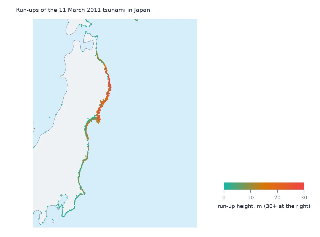
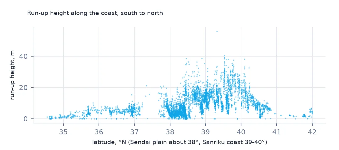
The highest run-ups are on the Iwate coast, 118 to 140 km from the source, where the wave funnelled into narrow bays. The top value, 55.9 m, is higher than the event's own maximum of 39.26 m. The two columns are kept separately, and the event figure is the one the compilers settled on. Use the run-up table for the pattern along the coast, and treat a single extreme point as a measurement to check.
2. Height against latitude
band = jp[jp.runupHt.notna()].groupby(jp.latitude.round(0)).runupHt.agg(["size", "median", "max"]).round(1)
print(band.loc[35:41].to_string())
size median max
latitude
35.0 107 1.2 4.8
36.0 225 4.0 10.1
37.0 292 5.0 21.1
38.0 1800 3.9 38.6
39.0 1453 13.0 55.9
40.0 880 14.2 40.6
41.0 210 5.6 11.5
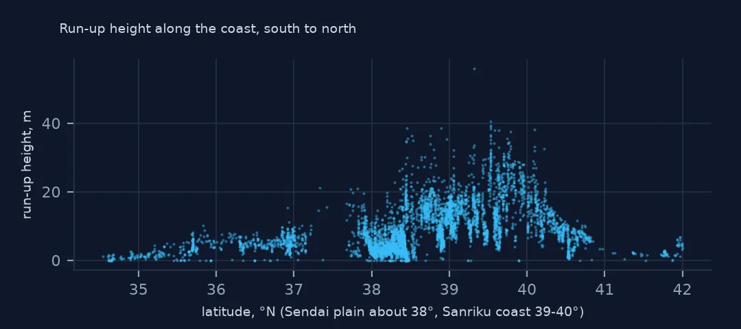
By degree of latitude, run-ups between 39° and 41° N, the Sanriku coast of Iwate, have medians of 13.0 and 14.2 m. At 38° N, the Sendai plain in Miyagi has the most run-ups, 1,800, but a median of 3.9 m: a flat coast where the water spread far inland without rising as high. South of 37° the heights fall off quickly.
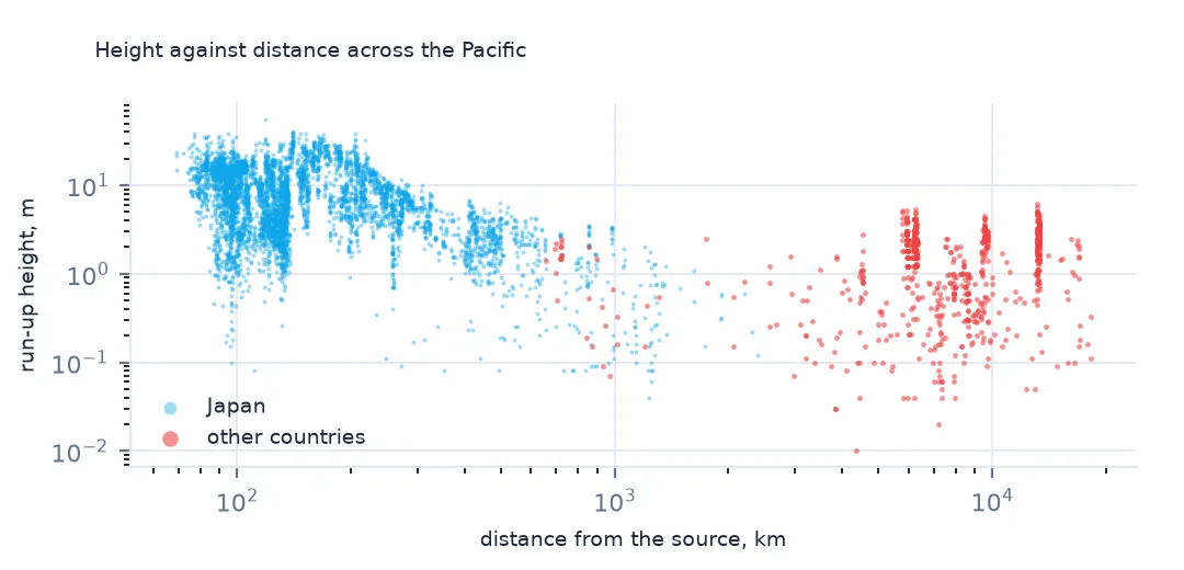
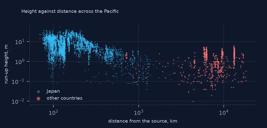
3. Height against distance
d = g[g.runupHt.notna() & (g.runupHt > 0)]
print(d.groupby(pd.cut(d.distFromSource, [0, 200, 500, 1000, 5000, 20000])).runupHt.agg(["size", "median"]).round(2).to_string())
size median
distFromSource
(0, 200] 3886 8.40
(200, 500] 1212 4.90
(500, 1000] 224 1.58
(1000, 5000] 132 0.46
(5000, 20000] 658 1.74
Heights fall with distance, from a median of 8.4 m within 200 km to 0.46 m at 1,000 to 5,000 km. Beyond 5,000 km the median rises again, to 1.74 m, because those run-ups are on the coasts of the Americas and Pacific islands where survey teams measured where the wave came ashore, while the closer ones in that range are mostly tide gauges.
The Pacific-wide record
The data used on this page
NOAA's Global Historical Tsunami Database from the National Centers for Environmental Information (doi:10.7289/V5PN93H7), public domain: every event and run-up from its HazEL API, downloaded on 19 October 2026 and saved on this site, because records are added and revised. Heights are in metres and distances in kilometres.
from pathlib import Path
import json
import zipfile

import geopandas as gpd
import numpy as np
import pandas as pd
import requests

Path("data").mkdir(exist_ok=True)
# NOAA NCEI Global Historical Tsunami Database (doi:10.7289/V5PN93H7): every event and every run-up from the HazEL API,
# with Natural Earth's 1:50m land and 1:110m countries. Saved 19 October 2026: events and run-ups are added and revised.
# Live: https://www.ngdc.noaa.gov/hazel/hazard-service/api/v1/tsunamis/events?page=1 (and .../runups), 200 a page
ARCHIVE = "ncei-tsunami-2026-10-19.zip"
if not Path(f"data/{ARCHIVE}").exists():
    Path(f"data/{ARCHIVE}").write_bytes(requests.get(f"https://data.spatialworkflow.io/{ARCHIVE}", timeout=600).content)
Z = zipfile.ZipFile(f"data/{ARCHIVE}")
ev = pd.DataFrame(json.loads(Z.read("tsunami-events.json")))
ru = pd.DataFrame(json.loads(Z.read("tsunami-runups.json")))
print(f"NCEI tsunami database: {len(ev):,} events, {len(ru):,} run-ups")
NCEI tsunami database: 3,138 events, 35,129 run-ups
Example 1: deaths recorded at run-ups
print(f"run-ups with deaths: {g.deaths.notna().sum()}; deaths summed over run-ups: {g.deaths.sum():,.0f}; event deaths: {tohoku.deaths:,.0f}")
print(g.groupby("country").deaths.sum().loc[lambda s: s > 0].to_string())
run-ups with deaths: 43; deaths summed over run-ups: 15,952; event deaths: 18,423
country
INDONESIA 1.0
JAPAN 15950.0
USA 1.0
Only 43 run-ups carry a death count, summing to 15,952 of the event's 18,423 deaths, 15,950 of them in Japan. One person died in Indonesia and one in the United States, in California. Deaths in the run-up table are recorded where they could be placed, so they are a partial geography of the toll.
Example 2: the map of Japan
Path("data/ne_50m_land.zip").write_bytes(Z.read("ne_50m_land.zip"))
land = gpd.read_file("data/ne_50m_land.zip")
ax = land.plot(color="#e5e7eb", figsize=(7, 8))
jp.plot(ax=ax, column="runupHt", cmap="YlOrRd", markersize=3, legend=True, vmax=30)
ax.set_xlim(138.5, 146); ax.set_ylim(34.5, 42)
print(f"Japanese run-ups drawn: {len(jp):,}")
Japanese run-ups drawn: 5,513
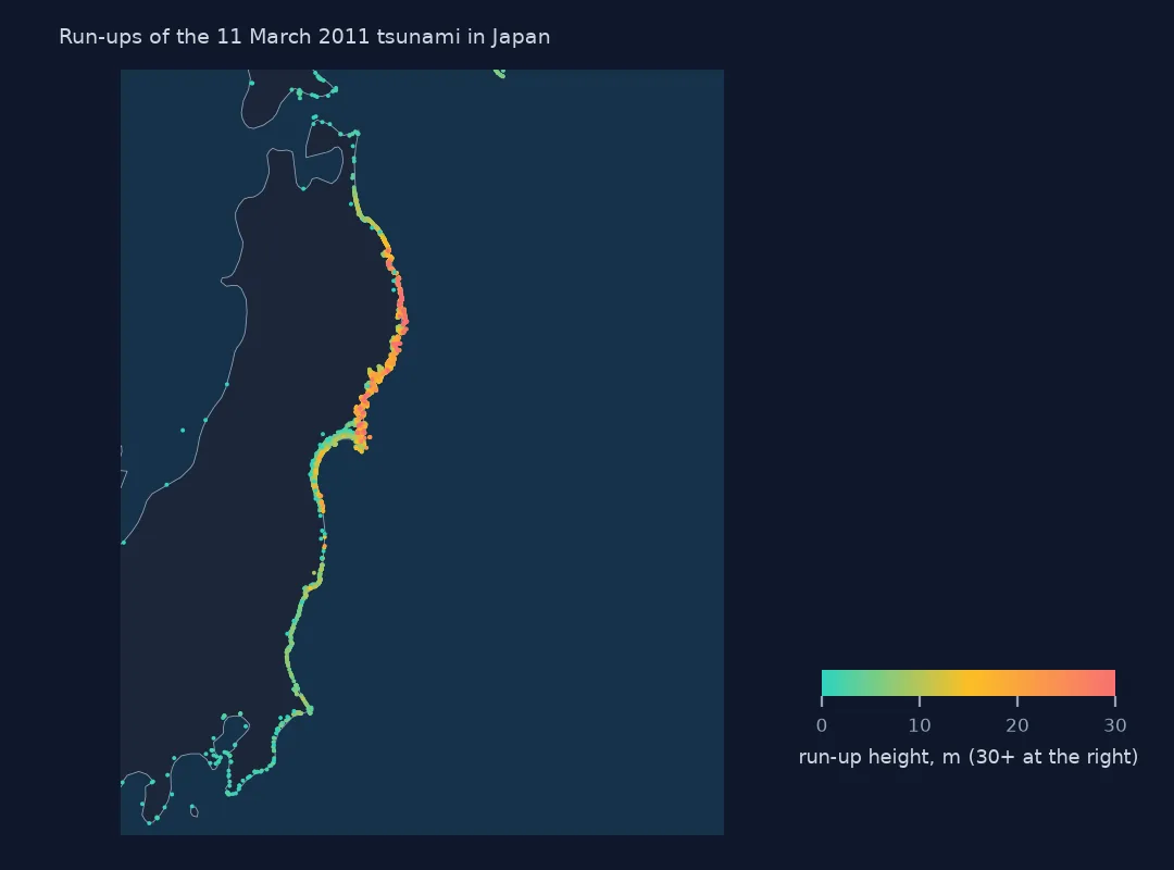
Within the map's frame the run-ups line the coast from southern Hokkaido to Chiba, with the tallest in red along the indented Sanriku coast of Iwate and northern Miyagi, and lower, densely surveyed points on the Sendai plain to the south.
Internal links
- Loading events and run-ups — the run-up table
- Travel times across the Pacific — the same event's arrivals far away
- The deadliest tsunamis — where 2011 ranks
- Every tsunami at one place — run-ups gathered by location instead