
How to Measure Cycling from Road Traffic Counts
On this page
Problem statement
Every manual traffic count in Britain records bicycles alongside cars and lorries, so the road traffic file is also one of the largest open records of cycling: thousands of locations a year since 2000. It is not a cycling survey, though. Most count points are on roads few people cycle on, the numbers are small and noisy, and the annual figure is expanded from one weekday in spring or autumn.
This page builds a cycling trend from the count points that were counted in consecutive years, shows how noise depends on the size of the count, compares London with the rest of Great Britain, and finds the busiest cycling roads — along with a duplicate that the file hides on a boundary.
Quick answer
Use only counted points with at least 20 cycles a day in both years, take the median year-on-year ratio, and chain:
a = aadf.sort_values(["count_point_id", "year"])
a["prev"] = a.groupby("count_point_id").pedal_cycles.shift()
a["prev_ok"] = (a.groupby("count_point_id").estimation_method.shift() == "Counted") & (a.groupby("count_point_id").year.shift() == a.year - 1)
pair = a[(a.estimation_method == "Counted") & a.prev_ok & (a.prev >= 20) & (a.pedal_cycles >= 20)]
step = pair.groupby("year").apply(lambda g: np.exp(np.log(g.pedal_cycles / g.prev).median()), include_groups=False)
index = (step.cumprod() * 100).reindex(range(2001, 2026))
print(f"{len(pair):,} counted pairs with 20+ cycles a day in both years")
print(index.loc[[2005, 2010, 2015, 2019, 2020, 2021, 2023, 2025]].round(1).to_string())
50,411 counted pairs with 20+ cycles a day in both years
year
2005 83.4
2010 91.5
2015 116.7
2019 117.8
2020 146.5
2021 130.5
2023 120.6
2025 128.6
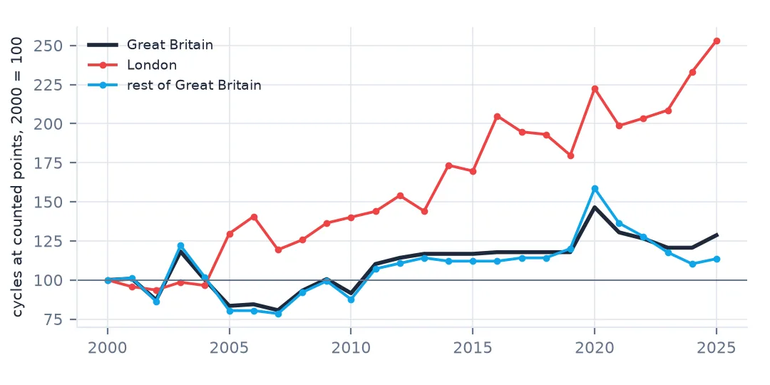
50,411 pairs give an index (2000 = 100) that dipped to 83.4 in 2005, was 116.7 by 2015 and 117.8 in 2019. In 2020 it jumped to 146.5, fell back to 120.6 by 2023 and was 128.6 in 2025: about a quarter more cycling than in 2000 on the roads where it is counted, but well below the pandemic peak.
Small counts, London and the rest
1. Most count points see very few cyclists
y = aadf[(aadf.year >= 2022) & (aadf.estimation_method == "Counted")]
print(y.pedal_cycles.describe(percentiles=[0.25, 0.5, 0.75, 0.9, 0.99]).round(0).to_string())
print(f"counted points with zero cycles: {(y.pedal_cycles == 0).mean():.1%}")
count 31379.0
mean 117.0
std 563.0
min 0.0
25% 2.0
50% 16.0
75% 56.0
90% 158.0
99% 2368.0
max 13988.0
counted points with zero cycles: 21.2%
A median counted point since 2022 sees 16 cyclists a day and a quarter of them 2 or fewer; 21.2% see none at all. The distribution is extremely skewed, with a 99th percentile of 2,368 and a maximum of 13,988. Totals and means are dominated by a handful of urban roads.
2. Small counts make noisy changes
a2 = a[(a.estimation_method == "Counted") & a.prev_ok & (a.prev > 0) & (a.pedal_cycles > 0)].copy()
a2["log_change"] = np.log(a2.pedal_cycles / a2.prev)
band = pd.cut(a2.prev, [0, 5, 20, 100, 500, 1e6])
print(a2.groupby(band, observed=True).log_change.agg(lambda s: s.quantile(0.75) - s.quantile(0.25)).round(2).to_string())
prev
(0.0, 5.0] 1.18
(5.0, 20.0] 0.98
(20.0, 100.0] 0.70
(100.0, 500.0] 0.51
(500.0, 1000000.0] 0.29
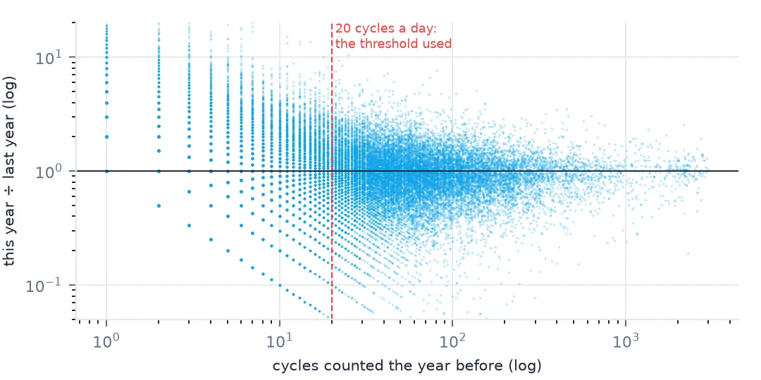
The year-to-year spread of a point's cycle count shrinks with its size: an interquartile range of 1.18 on the log scale for points with five or fewer cyclists — changes of a factor of three are routine — and 0.29 above 500. A single day's count of a handful of cyclists says little about trend; that is why the quick answer requires 20 in both years.
3. London and the rest
lon = {}
for name, g in pair.groupby(pair.region_name == "London"):
    s = g.groupby("year").apply(lambda h: np.exp(np.log(h.pedal_cycles / h.prev).median()), include_groups=False)
    lon["London" if name else "rest of Great Britain"] = (s.cumprod() * 100).reindex(range(2001, 2026))
lon = pd.DataFrame(lon)
print(lon.loc[[2010, 2015, 2019, 2020, 2025]].round(1).to_string())
rest of Great Britain London
year
2010 87.7 140.2
2015 112.0 169.7
2019 120.1 179.8
2020 158.6 222.4
2025 113.6 253.1
London and the rest of Great Britain have diverged. London's index reached 179.8 in 2019 and 253.1 in 2025 — cycling still growing after the pandemic. Outside London it rose to 120.1 by 2019, spiked to 158.6 in 2020 and has fallen back to 113.6, below its 2019 level.
4. Cyclists as a share of traffic
y25 = aadf[(aadf.year >= 2022) & (aadf.estimation_method == "Counted")]
share = y25.groupby(["region_name"]).apply(lambda g: g.pedal_cycles.sum() / (g.pedal_cycles.sum() + g.all_motor_vehicles.sum()), include_groups=False)
print((100 * share).sort_values(ascending=False).round(2).to_string())
region_name
London 2.85
South West 0.34
Yorkshire and The Humber 0.25
East of England 0.22
North West 0.21
East Midlands 0.20
South East 0.20
North East 0.19
West Midlands 0.17
Wales 0.17
Scotland 0.10
As a share of all traffic at counted points since 2022, cycles are 2.85% in London and 0.10–0.34% everywhere else. The South West, with 0.34%, is the next highest region — eight times lower than London.
The busiest roads, counted twice
The data used on this page
The Department for Transport's road traffic statistics: annual average daily flows (AADF) for every count point in Great Britain, 2000–2025, in the release of 2 June 2026, saved on this site because DfT revises earlier years with each release. Contains public sector information licensed under the Open Government Licence v3.0.
from pathlib import Path

import numpy as np
import pandas as pd
import requests

Path("data").mkdir(exist_ok=True)
# DfT republishes the counts every June and revises earlier years; this is the release of 2 June 2026
# (live: https://storage.googleapis.com/dft-statistics/road-traffic/downloads/data-gov-uk/dft_traffic_counts_aadf.zip).
AADF = "dft-traffic-counts-aadf-2026-06-02.zip"
if not Path(f"data/{AADF}").exists():
    Path(f"data/{AADF}").write_bytes(requests.get(f"https://data.spatialworkflow.io/{AADF}", timeout=600).content)
aadf = pd.read_csv(f"data/{AADF}", low_memory=False)
print(f"{len(aadf):,} rows, {aadf.count_point_id.nunique():,} count points, {aadf.year.min()}-{aadf.year.max()}")
600,551 rows, 46,754 count points, 2000-2025
Example 1: the busiest roads for cycling
top = y25.sort_values("pedal_cycles", ascending=False).drop_duplicates("count_point_id").head(6)
print(top[["year", "road_name", "local_authority_name", "pedal_cycles", "all_motor_vehicles"]].to_string(index=False))
year road_name local_authority_name pedal_cycles all_motor_vehicles
2023 A3 City of London 13988 9563
2023 A3 Southwark 13988 9563
2025 A201 City of London 13135 19217
2025 A201 City of London 13135 19217
2025 A201 Southwark 13135 19217
2025 A201 City of London 13063 15254
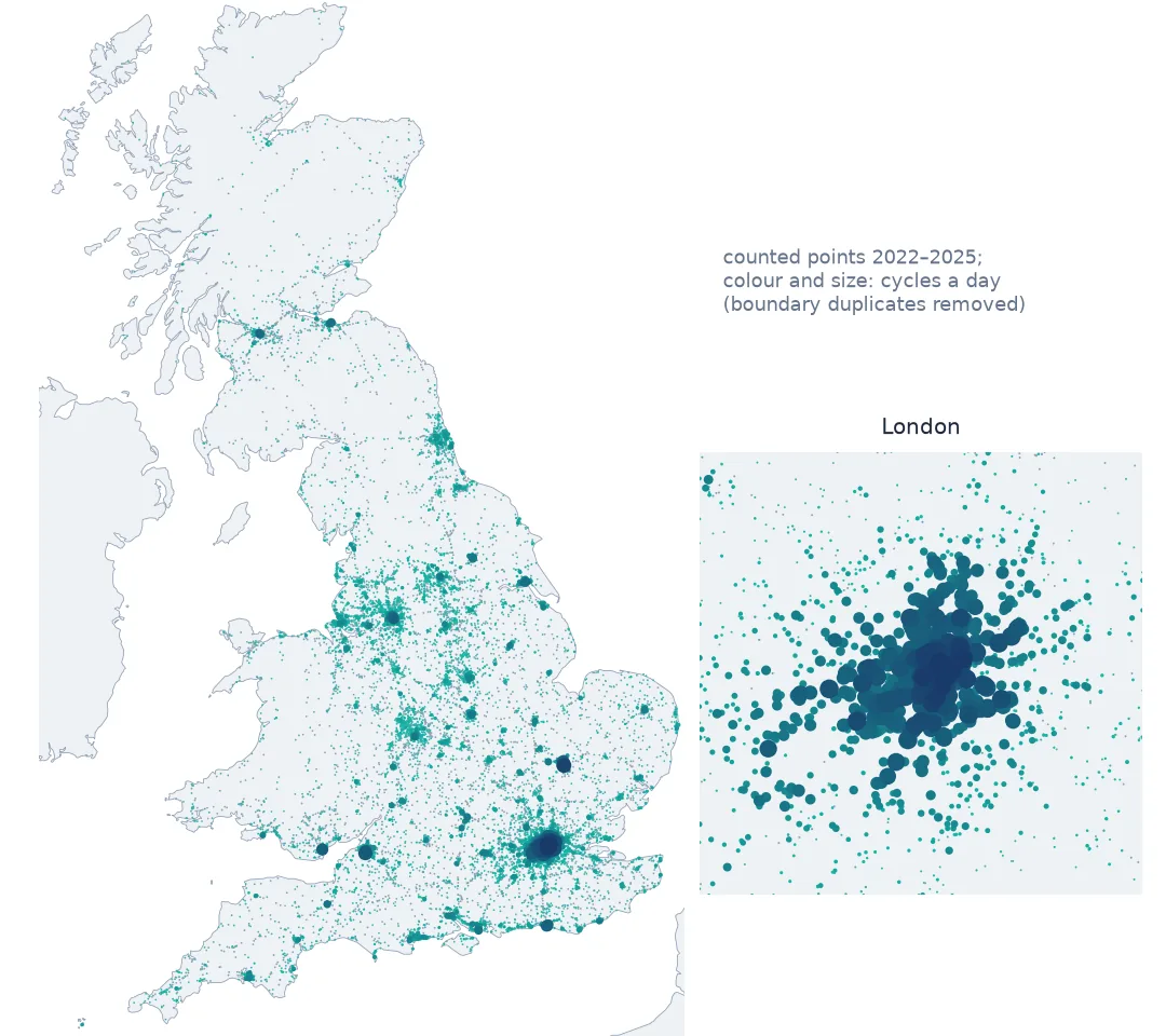
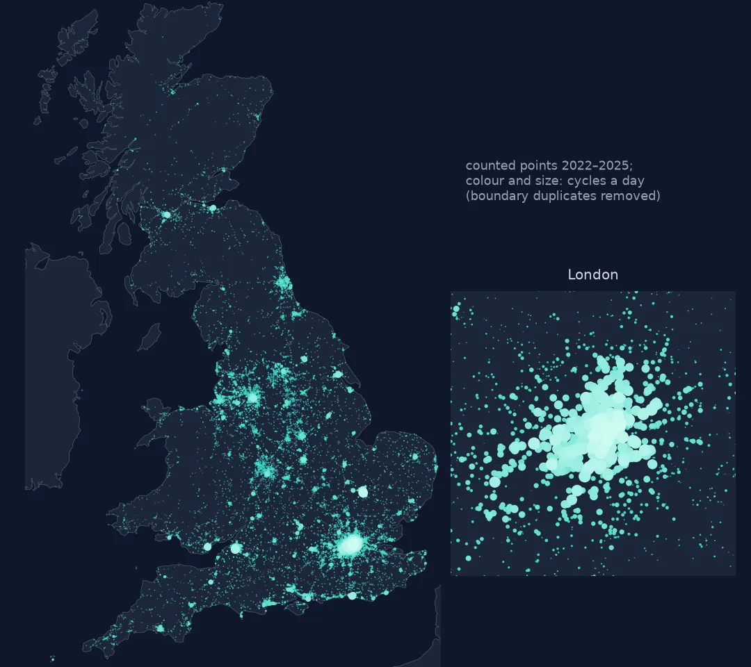
The busiest counted cycling roads are in central London, with 13,988 cyclists a day on the A3 in 2023 and 13,135 on the A201 in 2025 — more cyclists than motor vehicles on the first. The list shows a trap: each count appears twice, once for the City of London and once for Southwark, with identical figures under different count-point ids. The two authorities meet in the middle of the Thames, and a count on a road across the river is published for both. Deduplicate on road, year and values, not only on the id, before summing.
Example 2: weekday counts only
print("count points by year with a counted cycle figure:", a[a.estimation_method == "Counted"].groupby("year").size().loc[[2019, 2020, 2021, 2025]].to_dict())count points by year with a counted cycle figure: {2019: 13943, 2020: 7759, 2021: 8324, 2025: 7950}
The number of counted points also changes — 13,943 in 2019, 7,759 in 2020 — which is another reason to build the index from pairs rather than from yearly totals.
What a traffic count can say about cycling
A count point measures cycling where the road happens to be counted, which is not where most cycling happens: off-road paths, quiet back streets and parks are absent, and the minor-road sample is small. The index therefore describes cycling on the road network as DfT samples it. Its strength is breadth and continuity — the same method at thousands of places for 25 years — and its weakness is that a single weekday count of a small number of cyclists is a poor measurement, which the pairing and the 20-cycle threshold partly control.
The London result is robust to all of that: the gap with the rest of the country is large, consistent across years and present in the share of traffic as well as in the trend. Elsewhere, the post-pandemic fall below 2019 is a smaller signal on a noisier base, and worth checking against dedicated cycle counters before relying on it.
Pitfalls with cycle counts
- Small counts are noise. Require a minimum count in both years.
- Do not sum across boundary duplicates. The same count can appear under two authorities.
- Counts are weekday, daytime and seasonal. Weekend leisure cycling is under-represented.
- Expansion factors for cycles are assumed, not measured at the point.
- Counted points change every year; use pairs.
Internal links
- How to measure traffic trends from count points that were actually counted — the method for motor traffic
- How to build hour-of-day traffic profiles — when cyclists are counted
- How to clean a year of bike-share trip data — cycling from another source
- Annual average daily flow explained — expansion factors for cycles
FAQ
Has cycling increased in Great Britain?
At count points counted in consecutive years, cycling in 2025 stood at 128.6 on an index of 2000 = 100. In London it stood at 253.1; outside London at 113.6, below its 2019 level.
Where is the busiest cycling road in Britain?
In the DfT counts, central London: 13,988 cyclists a day on the A3 in 2023, counted on the boundary of the City of London and Southwark.