
Drought Indices Explained: Drought Monitor Categories, SPI and What Each Measures
On this page
Problem statement
"Drought" is reported as a US Drought Monitor category (D0 to D4), as a Standardized Precipitation Index (SPI) value, or as something else again, and the numbers do not agree: in Lincoln, Nebraska, the 12-month SPI was still below −1.9 in January 2013 while the 3-month SPI had recovered to −0.46. Neither index is wrong. They measure different things over different spans of time, and the Drought Monitor is not a single index at all but a weekly judgement that blends many. This page compares the two on 312 months of Lincoln's record, 2000–2025, to show what each one measures, how their categories line up, and when each is the right one to quote.
Quick answer
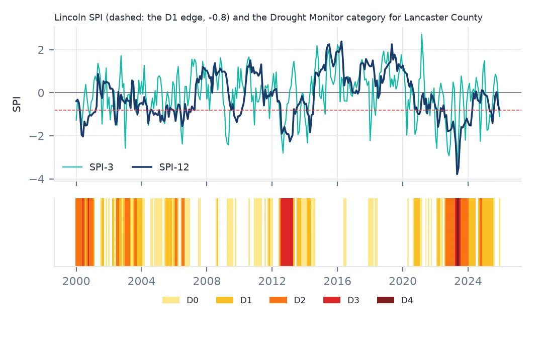
SPI measures one thing — how unusual the precipitation total over the last k months is for that time of year — and expresses it in standard deviations. The Drought Monitor category is a weekly expert classification that combines precipitation, soil moisture, streamflow and impacts. In Lincoln they agree in direction, and the Drought Monitor tracks the 12-month SPI more closely than the 3-month one.
p = monthly_precip("USW00014939")
spi3, spi12 = spi(p, 3), spi(p, 12)
lan = usdm_lan.set_index("MapDate")
dm = (lan[["D0", "D1", "D2", "D3", "D4"]] >= 50).sum(axis=1) - 1          # worst category covering half the county; -1 = none
dm_month = dm.resample("MS").max()
j = pd.DataFrame({"SPI-3": spi3, "SPI-12": spi12, "USDM": dm_month}).dropna()
print(f"{len(j)} months, 2000-2025, Lincoln, Nebraska")
print(j.corr(method="spearman").round(2).to_string())
312 months, 2000-2025, Lincoln, Nebraska
SPI-3 SPI-12 USDM
SPI-3 1.00 0.44 -0.47
SPI-12 0.44 1.00 -0.64
USDM -0.47 -0.64 1.00
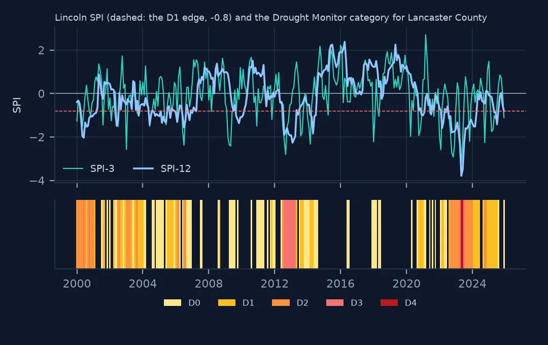
The rank correlation of the monthly Drought Monitor category with SPI-12 is −0.64, with SPI-3 −0.47: negative because a drier SPI is a lower number and a drier category a higher one. The two SPI scales correlate with each other at only 0.44.
SPI and the D categories side by side
1. Percentiles behind the D categories
cats = pd.DataFrame({"D category": ["D0", "D1", "D2", "D3", "D4"],
                     "percentile": ["21-30", "11-20", "6-10", "3-5", "0-2"],
                     "SPI": [-0.5, -0.8, -1.3, -1.6, -2.0]})
cats["SPI as a percentile"] = (100 * stats.norm.cdf(cats.SPI)).round(1)
print(cats.to_string(index=False))
D category percentile SPI SPI as a percentile
D0 21-30 -0.5 30.9
D1 11-20 -0.8 21.2
D2 6-10 -1.3 9.7
D3 3-5 -1.6 5.5
D4 0-2 -2.0 2.3
The Drought Monitor defines each category by the percentile of conditions it represents — D1 is roughly a 1-in-5 to 1-in-10 dryness, D4 rarer than 1 in 50 — and gives SPI ranges for each. Translated back through the normal distribution, the SPI cut-offs land close to the percentile bands: −0.8 is the 21.2th percentile, −2.0 the 2.3th. That is what lets an SPI value be read as a D category, as long as you remember SPI is only the precipitation part.
2. Same place, different index
print(j.loc["2012-04":"2013-03"].round(2).to_string()) SPI-3 SPI-12 USDM
2012-04-01 0.96 0.18 -1.0
2012-05-01 -0.41 -0.41 -1.0
2012-06-01 -0.48 -0.39 0.0
2012-07-01 -1.54 -0.54 2.0
2012-08-01 -2.14 -1.91 3.0
2012-09-01 -2.80 -1.76 3.0
2012-10-01 -1.58 -1.59 3.0
2012-11-01 -1.28 -1.84 3.0
2012-12-01 -0.53 -1.93 3.0
2013-01-01 -0.46 -1.93 3.0
2013-02-01 0.14 -2.27 3.0
2013-03-01 0.31 -2.12 3.0
The 2012 drought shows the time scales at work. SPI-3 went from +0.96 in April to −2.80 in September and was back above zero by February 2013. SPI-12 moved more slowly and stayed below −1.9 into 2013, because it still counted the dry summer. The Drought Monitor reached D3 in August and held it through March, much like SPI-12: soil moisture, reservoirs and groundwater had not recovered, whatever the last three months of rain said.
3. Time scale changes the answer
both_dry = ((j["SPI-3"] < -0.8) & (j["SPI-12"] < -0.8)).mean()
only3 = ((j["SPI-3"] < -0.8) & (j["SPI-12"] >= -0.8)).mean()
only12 = ((j["SPI-3"] >= -0.8) & (j["SPI-12"] < -0.8)).mean()
print(f"months dry (SPI < -0.8) on both scales: {both_dry:.1%}; on 3 months only: {only3:.1%}; on 12 months only: {only12:.1%}")
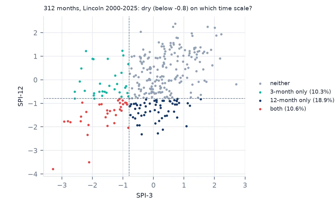
months dry (SPI < -0.8) on both scales: 10.6%; on 3 months only: 10.3%; on 12 months only: 18.9%
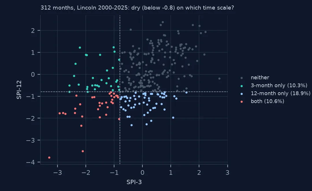
At a cut-off of −0.8 (the D1 edge), only 10.6% of months are dry on both scales. Another 10.3% are dry on the 3-month scale alone — short dry spells inside wet years — and 18.9% on the 12-month scale alone, long deficits that a wet season interrupted without erasing.
4. The Drought Monitor blends; SPI does not
ag = j.groupby("USDM")[["SPI-3", "SPI-12"]].median().round(2)
ag.index = ag.index.map(lambda k: "none" if k < 0 else f"D{k:.0f}")
print(ag.to_string())
SPI-3 SPI-12
USDM
none 0.50 0.67
D0 -0.06 -0.36
D1 -0.33 -0.69
D2 -0.55 -1.16
D3 -0.79 -1.93
D4 -2.71 -3.64
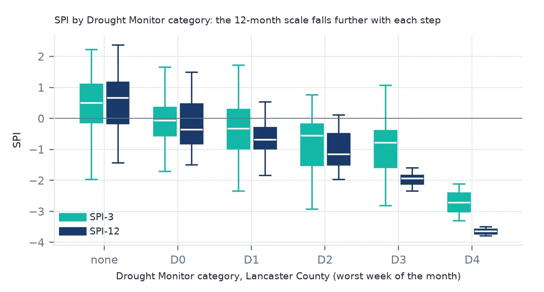
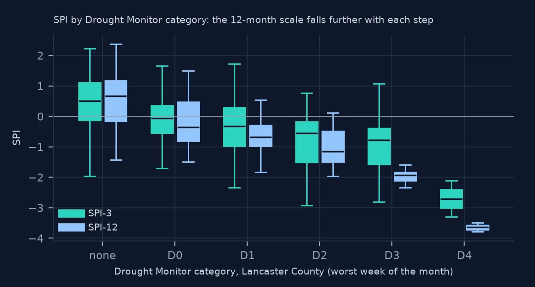
Grouped by the Drought Monitor's category, median SPI falls steadily with each step: SPI-12 goes from +0.67 in months with no drought to −1.16 in D2 and −3.64 in D4. SPI-3 falls less, and in D0 and D1 months it is barely negative (−0.06 and −0.33): a short wet spell does not lift the category, which is what you would expect from a classification that looks at long-term deficits.
How often each says drought, and which leads
The data used on this page
NOAA NCEI GHCN-Daily precipitation for Lincoln Municipal Airport, Nebraska (USW00014939), and the US Drought Monitor's weekly county statistics for Lancaster County, Nebraska, which contains Lincoln.
import io
from pathlib import Path

import numpy as np
import pandas as pd
import requests
from scipy import stats

Path("data").mkdir(exist_ok=True)
GHCN = "https://www.ncei.noaa.gov/data/global-historical-climatology-network-daily/access/{}.csv"
STATIONS = ["USW00014939"]                                                      # Lincoln, Nebraska
for sid in STATIONS:
    f = Path(f"data/{sid}.csv")
    if not f.exists():
        # the per-station files grow daily; this page uses complete months up to December 2025
        f.write_bytes(requests.get(GHCN.format(sid), timeout=300).content)


def monthly_precip(sid, min_days=25):
    d = pd.read_csv(f"data/{sid}.csv", usecols=["DATE", "PRCP", "PRCP_ATTRIBUTES"], parse_dates=["DATE"], low_memory=False)
    d = d[(d.DATE < "2026-01-01")]
    ok = d.PRCP_ATTRIBUTES.fillna(",,,").str.split(",").str[1] == ""            # drop quality-flagged values
    d = d.assign(mm=d.PRCP.where(ok) / 10).set_index("DATE")
    m = d.mm.resample("MS").agg(["sum", "count"])
    return m["sum"].where(m["count"] >= min_days)                                # a month needs 25 days of data


def spi(precip, scale, ref=("1991", "2020")):
    """Standardized Precipitation Index: gamma fit per calendar month on the reference period, with a point mass at zero."""
    acc = precip.rolling(scale).sum()
    out = pd.Series(np.nan, index=acc.index)
    for m in range(1, 13):
        sel = acc[acc.index.month == m]
        ref_vals = sel.loc[ref[0]:ref[1]].dropna()
        q = (ref_vals == 0).mean()
        a, _, b = stats.gamma.fit(ref_vals[ref_vals > 0], floc=0)
        out[sel.index] = stats.norm.ppf(q + (1 - q) * stats.gamma.cdf(sel, a, loc=0, scale=b))
    return out


r = requests.get("https://usdmdataservices.unl.edu/api/CountyStatistics/GetDroughtSeverityStatisticsByAreaPercent",
                 params={"aoi": "31109", "startdate": "1/1/2000", "enddate": "12/31/2025", "statisticsType": 1}, timeout=300)
usdm_lan = pd.read_csv(io.StringIO(r.text))                                        # Lancaster County, Nebraska
usdm_lan["MapDate"] = pd.to_datetime(usdm_lan.MapDate.astype(str), format="%Y%m%d")
print(f"Lancaster County: {len(usdm_lan):,} weekly maps")

for sid in STATIONS:
    m = monthly_precip(sid)
    print(f"{sid}: {m.notna().sum()} complete months, {m.first_valid_index():%Y-%m} to {m.last_valid_index():%Y-%m}")
Lancaster County: 1,357 weekly maps
USW00014939: 718 complete months, 1948-01 to 2025-12
Example 1: how often each index says "drought"
print(f"share of months: SPI-3 below -0.8 {(j['SPI-3'] < -0.8).mean():.1%}; SPI-12 below -0.8 {(j['SPI-12'] < -0.8).mean():.1%}; "
      f"Drought Monitor D1 or worse {(j.USDM >= 1).mean():.1%}")
share of months: SPI-3 below -0.8 20.8%; SPI-12 below -0.8 29.5%; Drought Monitor D1 or worse 33.0%
SPI-3 is below the D1 cut-off in 20.8% of months, close to the one in five the definition implies; SPI-12 in 29.5%, and the Drought Monitor puts at least half of Lancaster County in D1 or worse in 33.0% of months. 2000–2025 was drier on long time scales than the 1991–2020 baseline the SPI is fitted on — which is both what 2002, 2012 and 2022–2023 did and a reminder that the share depends on the reference period.
Example 2: lead and lag
for lag in [0, 1, 2, 3]:
    print(f"SPI-3 leading the Drought Monitor by {lag} months: rho = {j['SPI-3'].shift(lag).corr(j.USDM, method='spearman'):.2f}")
SPI-3 leading the Drought Monitor by 0 months: rho = -0.47
SPI-3 leading the Drought Monitor by 1 months: rho = -0.55
SPI-3 leading the Drought Monitor by 2 months: rho = -0.44
SPI-3 leading the Drought Monitor by 3 months: rho = -0.39
The correlation is strongest when SPI-3 leads by one month (−0.55), and weakens with longer lags. The Drought Monitor reacts to a dry spell, but a month late: its authors wait for the deficit to show in soils and streams before moving a category.
What each index is for
SPI is a transformation, not a model. It fits a probability distribution (a gamma, with a mass at zero) to the precipitation totals for each calendar month over a reference period, and maps each total to the standard normal value with the same probability. An SPI of −1.3 means "drier than all but about one in ten reference years for this time of year", at any station and any season, which is why it is the World Meteorological Organization's recommended meteorological drought index. Its time scale is the choice that matters: 1–3 months for soil moisture and crops, 6–12 for streams and reservoirs, 24 or more for groundwater.
The Drought Monitor is a different kind of object. Each week an author combines dozens of indicators — SPI at several scales, soil moisture models, streamflow percentiles, vegetation health, snowpack, and impact reports — and draws category boundaries on a map. Its percentile definitions make its categories comparable with SPI, but it can hold a category while precipitation recovers, as Lincoln's record shows in early 2013. Use SPI when you need a reproducible number you can compute anywhere and at any time scale; use the Drought Monitor when you need the official US drought status, as triggers for disaster aid and crop programmes do.
Pitfalls when comparing them
- Signs run opposite. Drier is a lower SPI and a higher D category; expect negative correlations.
- One station is not a county. Lincoln's airport gauge stands for Lancaster County here; the Drought Monitor's polygons draw on many stations and gridded data.
- Weekly against monthly. Comparing them needs a rule for the month, such as the worst weekly category of the month, used here; a different rule moves the numbers slightly.
- SPI says nothing about temperature. A hot summer with normal rain can dry soils quickly; indices with evaporation, such as SPEI, or soil-moisture percentiles catch that, and the Drought Monitor uses them.
Internal links
- How to calculate the SPI in Python — the index computed step by step
- How to analyse US Drought Monitor county statistics — the D categories by county
- SPI fails in dry climates — what happens with months of no rain
- How to analyse snow depth from GHCN-Daily — the same station files and flags
FAQ
Can I convert an SPI value to a Drought Monitor category?
As an approximation, yes, using the Drought Monitor's SPI ranges (−0.8 for D1, −1.3 for D2, −1.6 for D3, −2.0 for D4). It is only the precipitation part of the classification, so expect it to disagree with the official map whenever soils, streams or impacts tell a different story.
Which SPI time scale matches the Drought Monitor best?
In Lincoln over 2000–2025, SPI-12 (rank correlation −0.64) rather than SPI-3 (−0.47), which fits a classification built around long-term deficits.