
How to Relate Drought to River Flow: Precipitation Deficits and Low Flows
On this page
Problem statement
A precipitation deficit is the start of a drought, not the whole of it. Rivers respond later and more slowly, through soil moisture, groundwater and — on a managed river — reservoirs and irrigation, so the question "how dry is the river?" needs its own index and a way to connect it to the rainfall record. This guide reads 26,390 days of USGS discharge for the Platte River at Louisville, Nebraska, standardises monthly flow the way SPI standardises precipitation, and finds which precipitation time scale the river follows best.
Quick answer
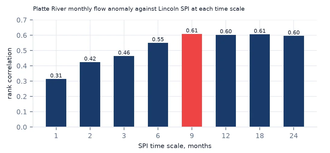
Average daily discharge to months, take logs, and standardise each calendar month against its 1991–2020 mean and spread. Then correlate the flow anomaly with SPI at several time scales and take the scale with the highest rank correlation: for the Platte at Louisville, around nine months.
p = monthly_precip("USW00014939")
q = flow.resample("MS").mean()
anom = np.log(q).groupby(q.index.month).transform(lambda x: (x - x.loc["1991":"2020"].mean()) / x.loc["1991":"2020"].std())
best = {}
for k in [1, 2, 3, 6, 9, 12, 18, 24]:
    best[k] = spi(p, k).corr(anom, method="spearman")
best = pd.Series(best)
print("rank correlation of monthly flow anomaly with SPI at each time scale:", best.round(2).to_dict())
print(f"strongest at {best.idxmax()} months")
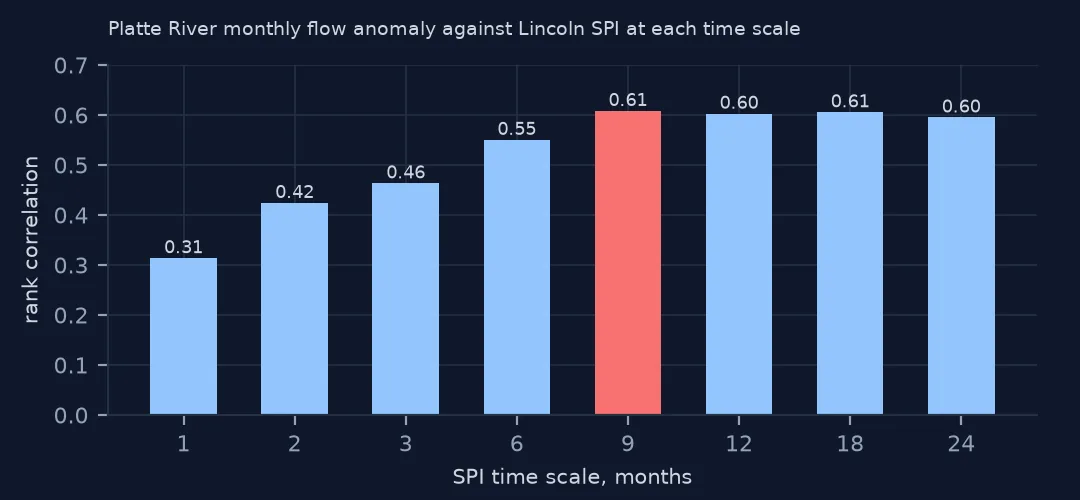
rank correlation of monthly flow anomaly with SPI at each time scale: {1: 0.31, 2: 0.42, 3: 0.46, 6: 0.55, 9: 0.61, 12: 0.6, 18: 0.61, 24: 0.6}
strongest at 9 months
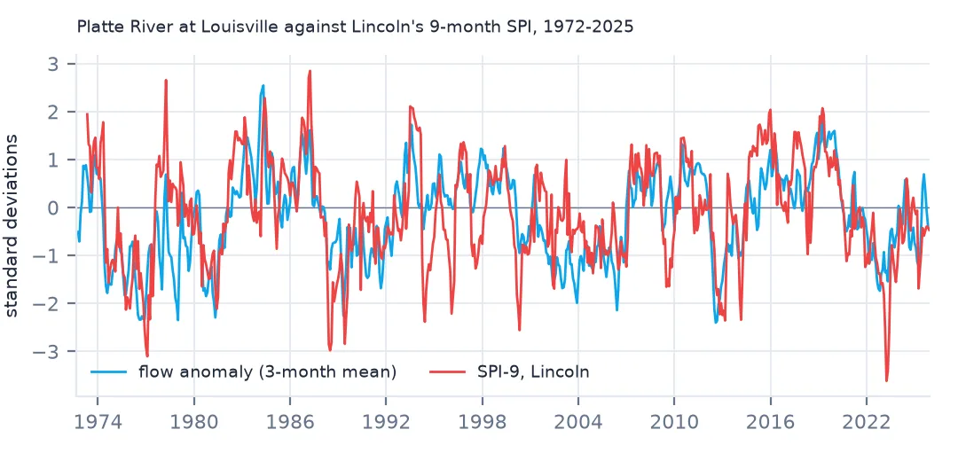
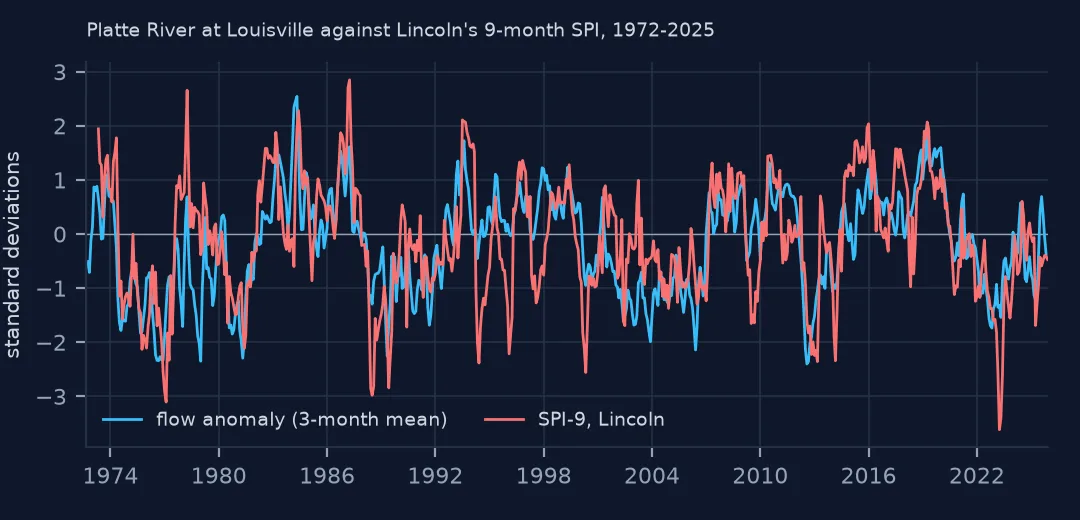
The correlation rises from 0.31 at one month to 0.61 at nine and stays near 0.6 out to two years. The river integrates rainfall over most of a year: a dry month barely moves it, a dry year does.
A flow anomaly for the Platte
1. Read the USGS daily values
print(f"{len(flow):,} days from {flow.index.min():%Y-%m-%d} to {flow.index.max():%Y-%m-%d}; median {flow.median():,.0f} cfs")
print("qualification codes:", raw_q.cd.value_counts().head(4).to_dict())
26,390 days from 1953-10-01 to 2025-12-31; median 5,820 cfs
qualification codes: {'A': 24179, 'A:e': 2211}
The record has 26,390 days from October 1953 with a median of 5,820 cfs. Every value is approved (A); 2,211 are approved estimates (A:e), typically days when ice or equipment problems made the gauge reading unusable. A drought study can keep them, but they are worth flagging.
2. Low-flow percentiles by season
pct = flow.groupby(flow.index.month).quantile([0.1, 0.5]).unstack()
print(pct.round(0).astype(int).T.to_string())
datetime 1 2 3 4 5 6 7 8 9 10 11 12
0.1 2251 3300 5181 4639 3711 3270 1360 1181 1400 2330 3260 2232
0.5 4500 6400 8475 7815 7875 8235 4850 3325 3600 4480 5250 4980
Flow has a strong season: the median is highest in March (8,475 cfs, snowmelt and spring rain) and lowest in August (3,325), when irrigation and evaporation take the most. The 10th percentile for August, 1,181 cfs, is a third of its median. A fixed low-flow threshold for the whole year would flag every August as drought; per-month percentiles avoid that.
3. Standardise flow like precipitation
print(f"flow anomaly 1991-2020: mean {anom.loc['1991':'2020'].mean():+.2f}, sd {anom.loc['1991':'2020'].std():.2f}")
print("driest months for the river:", anom.nsmallest(4).round(2).rename(lambda d: f"{d:%Y-%m}").to_dict())
flow anomaly 1991-2020: mean +0.00, sd 0.98
driest months for the river: {'1955-12': -4.11, '1955-11': -3.08, '1955-05': -3.03, '1955-08': -2.91}
Taking logs before standardising makes flow's skewed distribution closer to normal, so the anomaly behaves like SPI: mean 0.00 and spread 0.98 over the reference period. The four driest months for the river are all in 1955, during the 1950s drought, which was more severe on the Platte than anything since.
4. Does the river lag the rain?
s6 = spi(p, 6)
for lag in [0, 1, 2, 3, 6]:
    print(f"flow anomaly against SPI-6 from {lag} months earlier: rho {anom.corr(s6.shift(lag), method='spearman'):.2f}")
flow anomaly against SPI-6 from 0 months earlier: rho 0.55
flow anomaly against SPI-6 from 1 months earlier: rho 0.49
flow anomaly against SPI-6 from 2 months earlier: rho 0.43
flow anomaly against SPI-6 from 3 months earlier: rho 0.41
flow anomaly against SPI-6 from 6 months earlier: rho 0.33
Shifting SPI-6 earlier does not improve the fit: the correlation is highest with no lag (0.55) and falls to 0.33 at six months. The lag is already inside the index — a six-month total ending this month is mostly rain from earlier months — which is why longer SPI scales match the river better than shifted short ones.
Drought years and the long record
The data used on this page
USGS daily streamflow for the Platte River at Louisville, Nebraska, from the NWIS daily-values service, 1953–2025, read from a copy saved on this site because the legacy service is being retired; and NOAA NCEI GHCN-Daily precipitation for Lincoln, Nebraska (USW00014939), the nearest long record. The flow at Louisville reflects rain over a basin reaching into Colorado and Wyoming as well as Lincoln's, and upstream reservoirs and irrigation — the guide comes back to that.
from pathlib import Path
import numpy as np
import pandas as pd
import requests
from scipy import stats
Path("data").mkdir(exist_ok=True)
GHCN = "https://www.ncei.noaa.gov/data/global-historical-climatology-network-daily/access/{}.csv"
STATIONS = ["USW00014939"] # Lincoln, Nebraska
for sid in STATIONS:
f = Path(f"data/{sid}.csv")
if not f.exists():
# the per-station files grow daily; this page uses complete months up to December 2025
f.write_bytes(requests.get(GHCN.format(sid), timeout=300).content)
def monthly_precip(sid, min_days=25):
d = pd.read_csv(f"data/{sid}.csv", usecols=["DATE", "PRCP", "PRCP_ATTRIBUTES"], parse_dates=["DATE"], low_memory=False)
d = d[(d.DATE < "2026-01-01")]
ok = d.PRCP_ATTRIBUTES.fillna(",,,").str.split(",").str[1] == "" # drop quality-flagged values
d = d.assign(mm=d.PRCP.where(ok) / 10).set_index("DATE")
m = d.mm.resample("MS").agg(["sum", "count"])
return m["sum"].where(m["count"] >= min_days) # a month needs 25 days of data
def spi(precip, scale, ref=("1991", "2020")):
"""Standardized Precipitation Index: gamma fit per calendar month on the reference period, with a point mass at zero."""
acc = precip.rolling(scale).sum()
out = pd.Series(np.nan, index=acc.index)
for m in range(1, 13):
sel = acc[acc.index.month == m]
ref_vals = sel.loc[ref[0]:ref[1]].dropna()
q = (ref_vals == 0).mean()
a, _, b = stats.gamma.fit(ref_vals[ref_vals > 0], floc=0)
out[sel.index] = stats.norm.ppf(q + (1 - q) * stats.gamma.cdf(sel, a, loc=0, scale=b))
return out
# USGS NWIS daily mean discharge (cfs), Platte River at Louisville, NE; a frozen copy of
# https://waterservices.usgs.gov/nwis/dv/?format=rdb&sites=06805500¶meterCd=00060&startDT=1953-10-01&endDT=2025-12-31&statCd=00003
f = Path("data/usgs-06805500.rdb")
if not f.exists():
f.write_bytes(requests.get("https://data.spatialworkflow.io/usgs-nwis-06805500-daily-flow-2026-10-15.rdb", timeout=300).content)
raw_q = pd.read_csv(f, sep="\t", comment="#", dtype=str).iloc[1:] # second line holds field widths
raw_q = raw_q.rename(columns={"93576_00060_00003": "cfs", "93576_00060_00003_cd": "cd"})
raw_q["datetime"] = pd.to_datetime(raw_q.datetime)
flow = pd.to_numeric(raw_q.set_index("datetime").cfs, errors="coerce").dropna()
for sid in STATIONS:
m = monthly_precip(sid)
print(f"{sid}: {m.notna().sum()} complete months, {m.first_valid_index():%Y-%m} to {m.last_valid_index():%Y-%m}")USW00014939: 718 complete months, 1948-01 to 2025-12
Example 1: 2012 and 2022 at the river
for y in [2012, 2022]:
    lo = flow.loc[str(y)]
    print(f"{y}: lowest daily flow {lo.min():,.0f} cfs on {lo.idxmin():%d %b}; days below the all-record 10th percentile {(lo < flow.quantile(0.1)).sum()}")
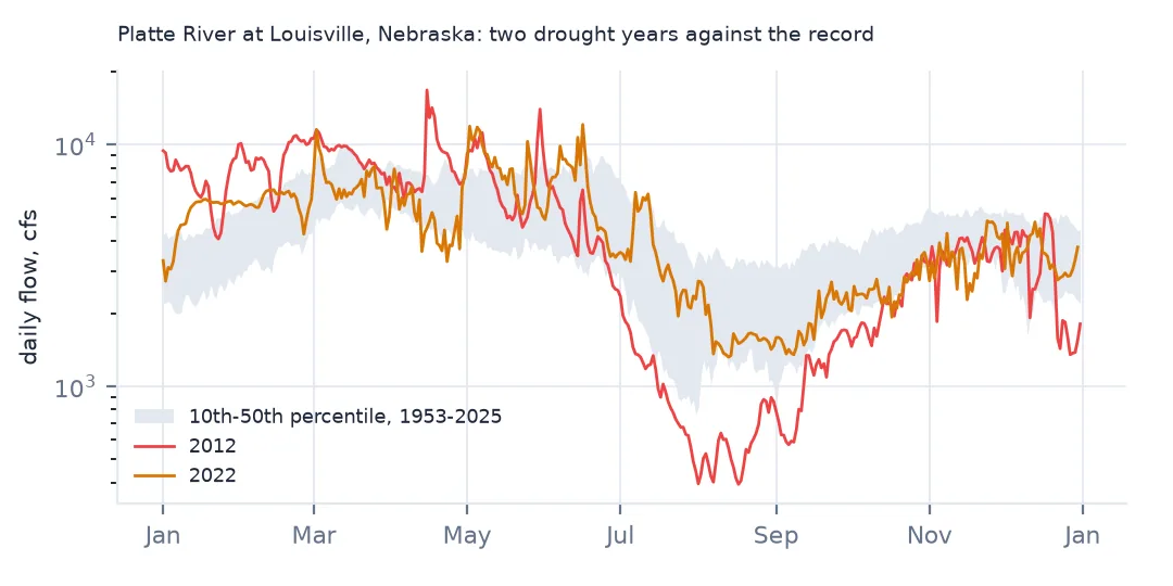
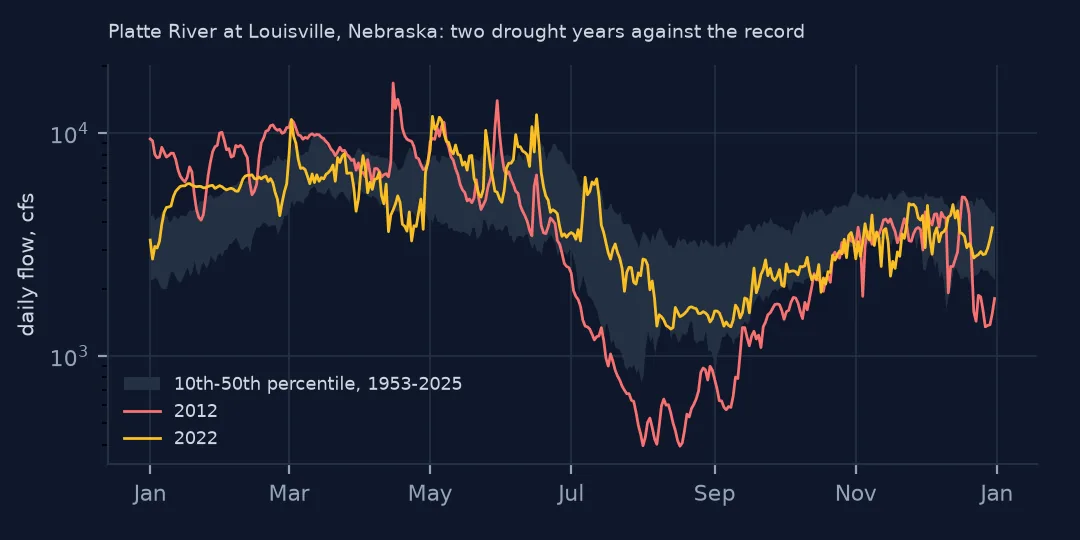
2012: lowest daily flow 393 cfs on 17 Aug; days below the all-record 10th percentile 122
2022: lowest daily flow 1,320 cfs on 14 Aug; days below the all-record 10th percentile 57
In 2012 the river fell to 393 cfs on 17 August and spent 122 days below the record's 10th percentile of daily flow; in 2022 the low was 1,320 cfs and 57 days. Both were drought years in Lancaster County, but the river's response differed by a factor of two: the flow at Louisville depends on the whole basin upstream, which one station's rainfall cannot describe.
Example 2: has the river got drier?
yr = flow.groupby(flow.index.year).median()
print(f"median annual flow by decade, cfs:", yr.groupby(yr.index // 10 * 10).median().round(0).astype(int).to_dict())
print(f"rank trend of annual median flow since 1954: {stats.spearmanr(yr.loc[1954:2025].index, yr.loc[1954:2025].values).statistic:+.2f}")
median annual flow by decade, cfs: {1950: 3690, 1960: 4170, 1970: 4425, 1980: 6525, 1990: 8165, 2000: 5020, 2010: 8350, 2020: 5860}
rank trend of annual median flow since 1954: +0.49
Median annual flow was lowest in the 1950s (3,690 cfs), higher from the 1980s (6,525) and 1990s (8,165), and has varied since — 5,020 in the 2000s, 8,350 in the 2010s. The rank trend since 1954 is +0.49: the river has got wetter, not drier, over the record, which changes what "low" means depending on the reference period.
Meteorological and hydrological drought
Precipitation deficits (meteorological drought) become low flows (hydrological drought) with a delay and a smoothing set by the catchment: how much water the soils and aquifers store, how fast they release it, and what people take out. The Platte at Louisville drains more than the Lincoln area — its basin reaches the Rocky Mountains — and its flow includes groundwater that has taken years to arrive, so a single station's SPI explains only part of it. A correlation of about 0.6 at nine months is a good result for that pairing.
Standardising flow per calendar month is the same idea as SPI, and published indices do it formally: the Standardized Streamflow Index fits a distribution to flow totals in the same way. The log transform used here is a simpler version that works for perennial rivers; a river that runs dry needs the zero-mass treatment SPI uses for rainless months.
What to watch on a managed river
- Regulation. Reservoir releases and irrigation diversions change flow independently of rain. Compare with an unregulated gauge, if there is one, before reading drought into the record.
- Trends in the baseline. The Platte's median flow has risen since the 1950s; a 1991–2020 reference treats the 1950s as extreme drought, and a 1951–1980 one would not.
- Gaps in the rainfall record. Lincoln's precipitation series has no data from 1954 to 1972, so correlations here use the months both series cover.
- Units. NWIS reports cubic feet per second; multiply by 0.0283 for cubic metres per second before comparing with other countries' data.
Internal links
- How to calculate the SPI in Python — the precipitation side
- Drought indices explained — meteorological against hydrological drought
- How to identify drought events from an index — events in either series
FAQ
Which SPI time scale should I compare with river flow?
Test several. For the Platte at Louisville the rank correlation was highest at nine months (0.61) and nearly as high from 12 to 24.
Where do I get USGS daily flow?
From the NWIS daily-values service as tab-separated RDB, or from its successor at api.waterdata.usgs.gov. Parameter 00060 is discharge and statistic 00003 the daily mean.