How to Calculate the Standardized Precipitation Index (SPI) in Python

Problem statement

The Standardized Precipitation Index (SPI) turns a precipitation total into a number of standard deviations from normal for that place, season and time scale, so that a dry summer in Nebraska and a dry winter in Oregon can be compared. Packages exist, but the method is short enough to write, and writing it shows the decisions a package makes for you: how to build monthly totals from daily records with gaps, which reference period to fit, and how to handle months with no rain. This guide computes SPI at 1, 3, 6 and 12 months from 718 complete months of daily records at Lincoln, Nebraska, and checks it against the 2012 drought.

Quick answer

Sum daily precipitation to months, take a rolling k-month total, fit a gamma distribution to each calendar month's totals over a reference period (1991–2020 here), and pass each total's gamma probability through the inverse normal. The spi() function in the setup does exactly that, with a probability mass for zero totals.

p = monthly_precip("USW00014939")
s3, s12 = spi(p, 3), spi(p, 12)
print(f"{p.notna().sum()} complete months from {p.first_valid_index():%Y-%m} to {p.last_valid_index():%Y-%m}")
print("driest 12 months on record:", f"{s12.idxmin():%B %Y}", f"SPI-12 = {s12.min():.2f}")
print("SPI-3 in 2012:", {f"{k:%b}": v for k, v in s3.loc["2012-05":"2012-10"].round(2).items()})

718 complete months from 1948-01 to 2025-12
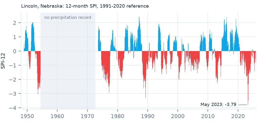
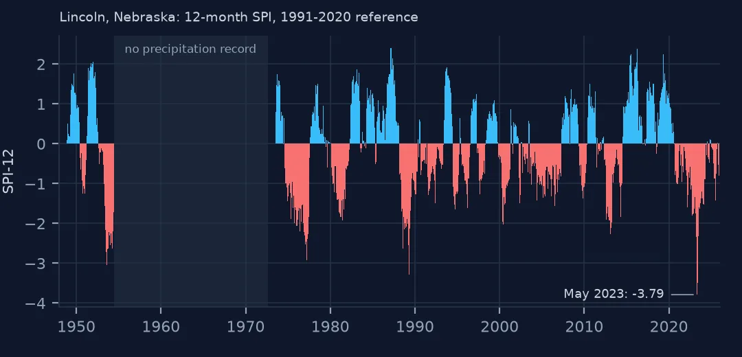
driest 12 months on record: May 2023 SPI-12 = -3.79
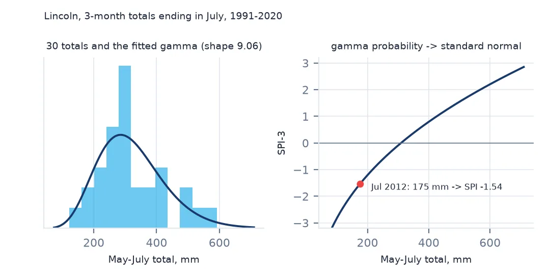
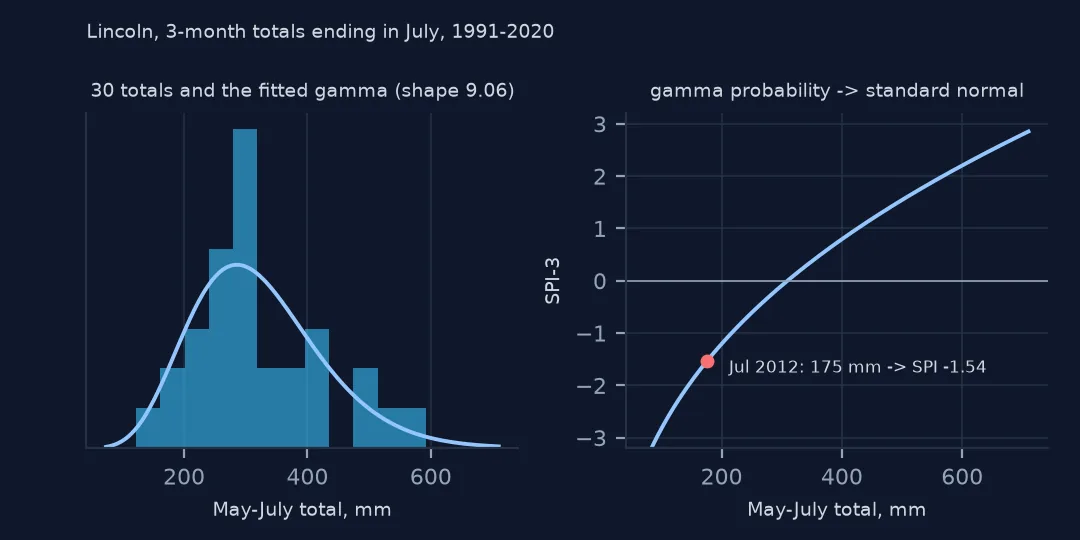
SPI-3 in 2012: {'May': -0.41, 'Jun': -0.48, 'Jul': -1.54, 'Aug': -2.14, 'Sep': -2.8, 'Oct': -1.58}

The driest 12 months in Lincoln's record end in May 2023, with an SPI-12 of −3.79 — drier than anything in the 1991–2020 reference period by a wide margin. In 2012 the 3-month SPI fell from −0.41 in May to −2.8 in September, the depth of that summer's flash drought.

From daily rain to SPI

1. Monthly totals from daily data

inside = p.loc[p.first_valid_index():]
print(f"months since {inside.index[0]:%Y-%m} with too few days to total: {inside.isna().sum()}; annual mean {p.loc['1991':'2020'].groupby(p.loc['1991':'2020'].index.year).sum().mean():.0f} mm")
gap = inside.isna()
run = (gap != gap.shift()).cumsum()[gap]
longest = inside[gap][run == run.value_counts().idxmax()]
print(f"longest gap: {longest.index[0]:%Y-%m} to {longest.index[-1]:%Y-%m}, {len(longest)} months")
print("mean by calendar month, 1991-2020, mm:", p.loc["1991":"2020"].groupby(p.loc["1991":"2020"].index.month).mean().round(0).astype(int).to_dict())

months since 1948-01 with too few days to total: 218; annual mean 745 mm
longest gap: 1954-07 to 1972-08, 218 months
mean by calendar month, 1991-2020, mm: {1: 19, 2: 23, 3: 39, 4: 68, 5: 125, 6: 114, 7: 83, 8: 84, 9: 74, 10: 54, 11: 33, 12: 30}

A month needs 25 days of unflagged values to get a total. Since January 1948, 218 months fail, and all of them are one gap: the airport station recorded no precipitation from July 1954 to August 1972. SPI is left blank there rather than filled from another station, which would change the series' statistics. The 1991–2020 means show Lincoln's climate: 745 mm a year, most of it from April to September, with May the wettest month at 125 mm.

2. Accumulate over the time scale

acc3 = p.rolling(3).sum()
print(f"3-month totals: {acc3.notna().sum()} values; {(acc3.isna() & p.notna()).sum()} months with data get none, because a month before them is blank")

3-month totals: 714 values; 4 months with data get none, because a month before them is blank

A 3-month total needs all three months; any blank month blanks the totals that include it. Here only 4 months with data lose their total, all at the edges of the gap.

3. Fit a gamma distribution per calendar month

fits = {}
for m in range(1, 13):
    v = acc3[acc3.index.month == m].loc["1991":"2020"].dropna()
    a, _, b = stats.gamma.fit(v[v > 0], floc=0)
    ks = stats.kstest(v[v > 0], "gamma", args=(a, 0, b)).pvalue
    fits[m] = (round(a, 2), round(b, 1), round(ks, 2))
print(pd.DataFrame(fits, index=["shape", "scale (mm)", "KS p-value"]).T.to_string())

    shape  scale (mm)  KS p-value
1    4.87        16.7        0.45
2    4.72        15.0        0.93
3    6.51        12.4        0.60
4   12.54        10.4        0.56
5    6.90        33.7        0.96
6   10.75        28.5        0.85
7    9.06        35.4        0.71
8    7.41        37.9        0.67
9    6.81        35.3        0.75
10   6.66        31.8        0.82
11   8.88        18.1        0.93
12   7.21        16.3        0.68

Each calendar month gets its own gamma fit, because a 3-month total ending in January (winter, mostly snow) and one ending in July (the wettest season) have different distributions: the scale parameter runs from 10.4 mm for April to 37.9 mm for August. A Kolmogorov–Smirnov test finds no month where the gamma fit is rejected; the lowest p-value is 0.45, for January. (The test is approximate, because the parameters come from the same data.)

4. Transform to a standard normal

ref = s3.loc["1991":"2020"]
print(f"SPI-3 over the reference period: mean {ref.mean():+.2f}, sd {ref.std():.2f}, below -1.3 in {(ref < -1.3).mean():.1%} of months")
print(f"whole record: below -1.3 in {(s3 < -1.3).mean():.1%} of months")

SPI-3 over the reference period: mean +0.00, sd 1.00, below -1.3 in 10.8% of months
whole record: below -1.3 in 10.2% of months

Over the reference period SPI-3 has mean 0.00 and standard deviation 1.00, as it should by construction, and it falls below −1.3 (the D2 cut-off) in 10.8% of months, close to the 10% a normal distribution gives. Over the whole record the share is 10.2%.

The reference period and the time scale

The data used on this page

NOAA NCEI GHCN-Daily precipitation for Lincoln Municipal Airport, Nebraska (USW00014939), with quality-flagged values removed and months with fewer than 25 days of data left blank.

from pathlib import Path

import numpy as np
import pandas as pd
import requests
from scipy import stats

Path("data").mkdir(exist_ok=True)
GHCN = "https://www.ncei.noaa.gov/data/global-historical-climatology-network-daily/access/{}.csv"
STATIONS = ["USW00014939"]                                                      # Lincoln, Nebraska
for sid in STATIONS:
    f = Path(f"data/{sid}.csv")
    if not f.exists():
        # the per-station files grow daily; this page uses complete months up to December 2025
        f.write_bytes(requests.get(GHCN.format(sid), timeout=300).content)


def monthly_precip(sid, min_days=25):
    d = pd.read_csv(f"data/{sid}.csv", usecols=["DATE", "PRCP", "PRCP_ATTRIBUTES"], parse_dates=["DATE"], low_memory=False)
    d = d[(d.DATE < "2026-01-01")]
    ok = d.PRCP_ATTRIBUTES.fillna(",,,").str.split(",").str[1] == ""            # drop quality-flagged values
    d = d.assign(mm=d.PRCP.where(ok) / 10).set_index("DATE")
    m = d.mm.resample("MS").agg(["sum", "count"])
    return m["sum"].where(m["count"] >= min_days)                                # a month needs 25 days of data


def spi(precip, scale, ref=("1991", "2020")):
    """Standardized Precipitation Index: gamma fit per calendar month on the reference period, with a point mass at zero."""
    acc = precip.rolling(scale).sum()
    out = pd.Series(np.nan, index=acc.index)
    for m in range(1, 13):
        sel = acc[acc.index.month == m]
        ref_vals = sel.loc[ref[0]:ref[1]].dropna()
        q = (ref_vals == 0).mean()
        a, _, b = stats.gamma.fit(ref_vals[ref_vals > 0], floc=0)
        out[sel.index] = stats.norm.ppf(q + (1 - q) * stats.gamma.cdf(sel, a, loc=0, scale=b))
    return out


for sid in STATIONS:
    m = monthly_precip(sid)
    print(f"{sid}: {m.notna().sum()} complete months, {m.first_valid_index():%Y-%m} to {m.last_valid_index():%Y-%m}")

USW00014939: 718 complete months, 1948-01 to 2025-12

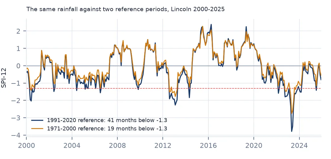
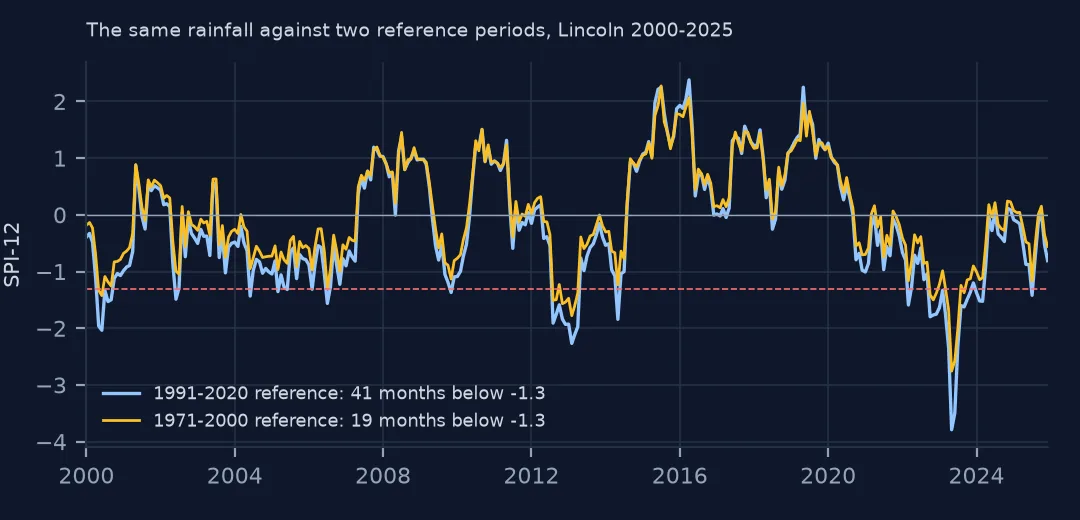
Example 1: the reference period matters

alt = spi(p, 12, ref=("1971", "2000"))
print(f"SPI-12 for September 2012: {s12.loc['2012-09-01']:.2f} with a 1991-2020 reference, {alt.loc['2012-09-01']:.2f} with 1971-2000")
print(f"months below -1.3 since 2000: {(s12.loc['2000':] < -1.3).sum()} (1991-2020 base) against {(alt.loc['2000':] < -1.3).sum()} (1971-2000 base)")

SPI-12 for September 2012: -1.76 with a 1991-2020 reference, -1.50 with 1971-2000
months below -1.3 since 2000: 41 (1991-2020 base) against 19 (1971-2000 base)

The same September 2012 is −1.76 against 1991–2020 and −1.50 against 1971–2000. Since 2000 the newer reference finds 41 months below −1.3 and the older one 19: 1991–2020 was wetter at the 12-month scale, so the same dry spell looks more unusual against it. SPI is relative to its reference; quote the period with the number.

Example 2: four time scales, one year

tab = pd.DataFrame({f"SPI-{k}": spi(p, k) for k in (1, 3, 6, 12)}).loc["2012-01":"2012-12"]
print(tab.round(2).to_string())

            SPI-1  SPI-3  SPI-6  SPI-12
DATE                                   
2012-01-01  -1.91   0.29   0.37   -0.15
2012-02-01   1.58   0.88  -0.46    0.09
2012-03-01  -0.46   0.11  -0.12    0.14
2012-04-01   0.75   0.96   0.72    0.18
2012-05-01  -0.64  -0.41  -0.07   -0.41
2012-06-01  -0.09  -0.48  -0.48   -0.39
2012-07-01  -2.13  -1.54  -1.05   -0.54
2012-08-01  -2.59  -2.14  -2.10   -1.91
2012-09-01  -0.59  -2.80  -1.91   -1.76
2012-10-01   0.17  -1.58  -2.10   -1.59
2012-11-01  -1.44  -1.28  -2.30   -1.84
2012-12-01   0.57  -0.53  -2.55   -1.93

Through 2012, SPI-1 swings month to month (−1.91 in January, +1.58 in February); SPI-3 picks up the summer deficit from July; SPI-6 is at its lowest in December (−2.55), because by then it spans the whole dry half-year; SPI-12 is still near −1.9 in December. Each scale answers a different question, which is why drought reports quote more than one.

Why a gamma, and why per month

Precipitation totals are bounded at zero and skewed: most months are near the median and a few are very wet. A two-parameter gamma distribution fits that shape well for totals of a month or more, which is why McKee, Doesken and Kleist chose it when they defined SPI in 1993. Fitting each calendar month separately removes the seasonal cycle; without that, every winter would look like a drought.

The inverse-normal step is what makes SPI comparable across places: whatever the shape of the local distribution, an SPI of −1.3 is a total that only about one month in ten falls below. When some totals are zero, the probability is q + (1 − q) · G(x), where q is the share of zeros in the reference period. In a wet climate like Lincoln's that mass is never used; in a desert it decides the result, as SPI fails in dry climates shows.

Before you trust the numbers

• Thirty years of reference, at least. With fewer, each month's gamma rests on a handful of values and extreme SPI values become unreliable. The WMO recommends 30 years; Lincoln's gap is why its earlier reference periods are shorter than they look.
• Quality flags. GHCN-Daily marks suspect values in PRCP_ATTRIBUTES; dropping them (as the setup does) and counting the days that remain is safer than treating a missing day as dry.
• Extreme values beyond ±3 come from the tails of a fitted distribution, where there is little data. Report them as "below −3", not as precise numbers.
• Station moves. An airport gauge can change site or instrument; GHCN's station history is worth a look before reading trends from the index.

Internal links

• Drought indices explained — SPI against the Drought Monitor
• SPI fails in dry climates — months with no rain
• How to identify drought events from an index — from SPI to events
• How to analyse snow depth from GHCN-Daily — the station files and their flags

FAQ

Which reference period should I use?

The current WMO normal, 1991–2020, unless you need to match a published series. Changing it moved Lincoln's September 2012 SPI-12 from −1.76 to −1.50, so always state it.

Is there a package that does this?

Yes — climate_indices and standard_precip implement SPI, with options for the fitting method. Writing it out, as here, makes the choices visible; check a package's defaults for the reference period and zero handling before comparing results.