
How to Count the People Living in Drought: Area-Weighted Against Population-Weighted
On this page
Problem statement
"A third of the country is in drought" usually means a third of the land area. Most of that land is thinly populated, so the share of people living in drought can be quite different — lower when the drought sits on the Plains and the deserts, higher when it reaches California or the cities of the East. Getting the people figure needs county population and an assumption about how people are spread within each county. This guide weights the Drought Monitor's weekly county shares by the Census Bureau's 2024 estimates, compares the result with the land share and with the Drought Monitor's own population statistics, and finds the weeks the two measures part most.
Quick answer
Join the county-week D1 share (cumulative, so D1 or worse) to county population and land area by FIPS code, multiply each by the share, and sum by week.
d = usdm.merge(pop, on="FIPS", how="inner").merge(area, on="FIPS", how="inner")
d["people_d1"] = d.pop2024 * d.D1 / 100
d["km2_d1"] = d.land_km2 * d.D1 / 100
wk = d.groupby("MapDate").agg(people=("people_d1", "sum"), km2=("km2_d1", "sum"))
wk["% of people"] = 100 * wk.people / pop.pop2024.sum()
wk["% of land"] = 100 * wk.km2 / area.land_km2.sum()
print(wk[["% of people", "% of land"]].describe().loc[["mean", "50%", "max"]].round(1).to_string())
print(f"weeks where the land share exceeds the population share: {(wk['% of land'] > wk['% of people']).mean():.0%}")
% of people % of land
mean 23.2 31.3
50% 23.4 30.5
max 51.6 65.7
weeks where the land share exceeds the population share: 80%
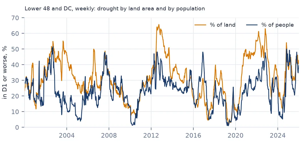
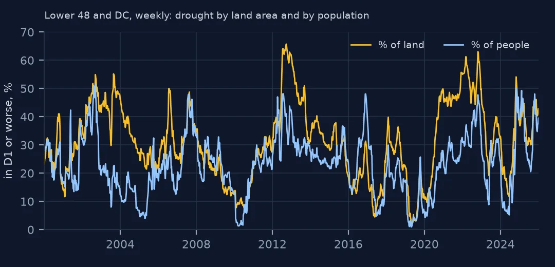
From 2000 to 2025 an average week had 31.3% of the land of the lower 48 and DC in D1 or worse, but 23.2% of the people. The land share was the larger in 80% of weeks. The peaks differ too: 65.7% of the land at most, 51.6% of the population.
Weighting the weekly shares by people
1. Population per county
print(f"{len(pop):,} counties, {pop.pop2024.sum():,} people (2024 estimates) in the lower 48 and DC")
print(f"half the population lives in the {(pop.pop2024.sort_values(ascending=False).cumsum() < pop.pop2024.sum() / 2).sum() + 1} most populous counties")
3,109 counties, 337,924,709 people (2024 estimates) in the lower 48 and DC
half the population lives in the 144 most populous counties
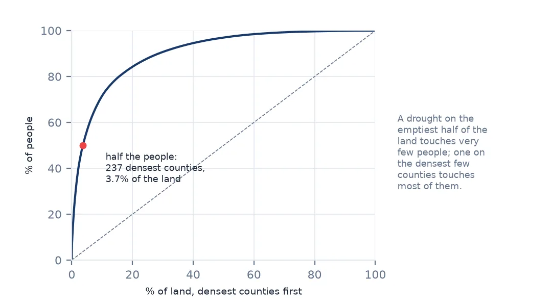
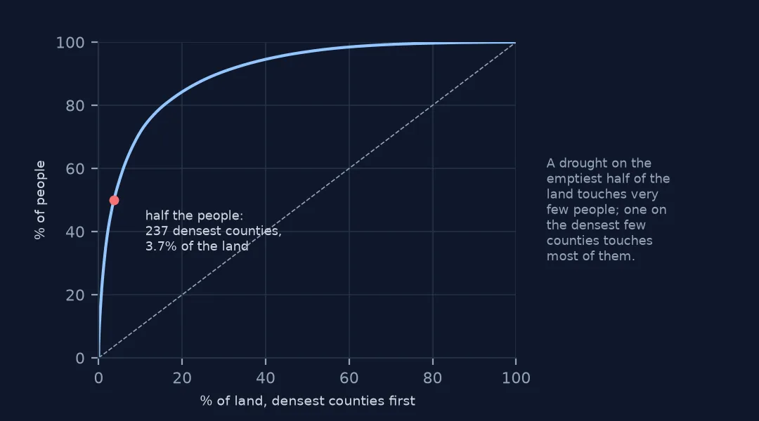
The 3,109 counties hold 337,924,709 people in the 2024 estimates, and half of them live in just 144 counties. Population is far more concentrated than land, which is why the two weightings disagree.
2. Land area per county
print(f"land area: {area.land_km2.sum():,.0f} km2; median county {area.land_km2.median():,.0f} km2")
print(f"counties matched by FIPS to the drought file: {usdm.FIPS.drop_duplicates().isin(pop.FIPS).mean():.1%}")
land area: 7,655,549 km2; median county 1,581 km2
counties matched by FIPS to the drought file: 100.0%
Land area comes from ALAND in the boundary file, which excludes water — the Great Lakes counties would otherwise count lake surface as land in drought. Every drought county matches a population row by FIPS.
3. Assume people are spread evenly within a county
row = d[(d.FIPS == "06037") & (d.MapDate == "2022-08-30")][["County", "D1", "pop2024", "people_d1"]]
print(row.to_string(index=False))
County D1 pop2024 people_d1
Los Angeles County 100.0 9757179 9757179.0
Within a county the method assumes people are spread evenly, so the share of a county in D1 is also the share of its people in D1. For Los Angeles County on 30 August 2022 the whole county was in D1 or worse, so all 9,757,179 residents count. Where a drought boundary cuts through a big county, the assumption can be badly wrong in either direction; a finer population grid, or census tracts, is the fix.
4. Compare with the Drought Monitor's own population statistics
off = usp.set_index("MapDate").join(wk)
off["gap"] = off["% of people"] - off.D1
print(f"our county-level estimate minus the official population-weighted D1 share: median {off.gap.median():+.1f} points, "
      f"90% within {off.gap.abs().quantile(0.9):.1f}")
our county-level estimate minus the official population-weighted D1 share: median +0.3 points, 90% within 1.2
The Drought Monitor publishes its own population-weighted statistics, built from finer population data. The county-level estimate is close: a median difference of +0.3 percentage points, and within 1.2 points in nine weeks out of ten. For national figures, county weighting is enough.
When the measures part and where the people are
The data used on this page
The US Drought Monitor's weekly county statistics (cumulative, 2000–2025) and its national population-weighted statistics; Census Bureau county population estimates for July 2024 (co-est2024-alldata.csv) and 2023 cartographic boundary counties for land area.
import io
from pathlib import Path

import geopandas as gpd
import numpy as np
import pandas as pd
import requests

Path("data").mkdir(exist_ok=True)
API = "https://usdmdataservices.unl.edu/api"
STATES = ["AL", "AZ", "AR", "CA", "CO", "CT", "DE", "DC", "FL", "GA", "ID", "IL", "IN", "IA", "KS", "KY", "LA", "ME", "MD",
          "MA", "MI", "MN", "MS", "MO", "MT", "NE", "NV", "NH", "NJ", "NM", "NY", "NC", "ND", "OH", "OK", "OR", "PA", "RI",
          "SC", "SD", "TN", "TX", "UT", "VT", "VA", "WA", "WV", "WI", "WY"]
for st in STATES:
    f = Path(f"data/usdm-county-{st}.csv")
    if not f.exists():
        # statisticsType 1 = cumulative percent of each county's area in each category or worse
        r = requests.get(f"{API}/CountyStatistics/GetDroughtSeverityStatisticsByAreaPercent",
                         params={"aoi": st, "startdate": "1/1/2000", "enddate": "12/31/2025", "statisticsType": 1}, timeout=600)
        f.write_text(r.text)
usdm = pd.concat([pd.read_csv(f"data/usdm-county-{st}.csv", dtype={"FIPS": str}) for st in STATES], ignore_index=True)
usdm["MapDate"] = pd.to_datetime(usdm.MapDate.astype(str), format="%Y%m%d")
for name, url in {"cb_2023_us_county_20m.zip": "https://www2.census.gov/geo/tiger/GENZ2023/shp/cb_2023_us_county_20m.zip"}.items():
    if not Path(f"data/{name}").exists():
        Path(f"data/{name}").write_bytes(requests.get(url, timeout=300).content)
f = Path("data/co-est2024-alldata.csv")
if not f.exists():
    f.write_bytes(requests.get("https://www2.census.gov/programs-surveys/popest/datasets/2020-2024/counties/totals/co-est2024-alldata.csv", timeout=300).content)
pop = pd.read_csv(f, encoding="latin-1", dtype={"STATE": str, "COUNTY": str})
pop = pop[(pop.SUMLEV == 50) & ~pop.STATE.isin(["02", "15"])]
pop = pd.DataFrame({"FIPS": pop.STATE + pop.COUNTY, "pop2024": pop.POPESTIMATE2024})
shapes = gpd.read_file("data/cb_2023_us_county_20m.zip")
shapes = shapes[~shapes.STATEFP.isin(["02", "15", "72"])]
area = pd.DataFrame({"FIPS": shapes.GEOID, "land_km2": shapes.ALAND / 1e6})
r = requests.get(f"{API}/USStatistics/GetDroughtSeverityStatisticsByPopulationPercent",
                 params={"aoi": "conus", "startdate": "1/1/2000", "enddate": "12/31/2025", "statisticsType": 1}, timeout=300)
usp = pd.read_csv(io.StringIO(r.text))                                             # the service's population-weighted shares
usp["MapDate"] = pd.to_datetime(usp.MapDate.astype(str), format="%Y%m%d")
print(f"{len(usdm):,} county-weeks, {usdm.FIPS.nunique():,} counties, {usdm.MapDate.nunique():,} weekly maps, "
      f"{usdm.MapDate.min():%Y-%m-%d} to {usdm.MapDate.max():%Y-%m-%d}")
4,218,913 county-weeks, 3,109 counties, 1,357 weekly maps, 2000-01-04 to 2025-12-30
Example 1: the weeks the two measures disagree most
wk["diff"] = wk["% of people"] - wk["% of land"]
print(wk.nlargest(3, "diff")[["% of people", "% of land"]].round(1).to_string())
print(wk.nsmallest(3, "diff")[["% of people", "% of land"]].round(1).to_string())
% of people % of land
MapDate
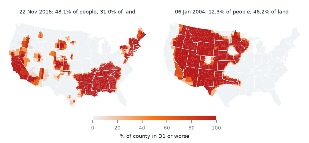
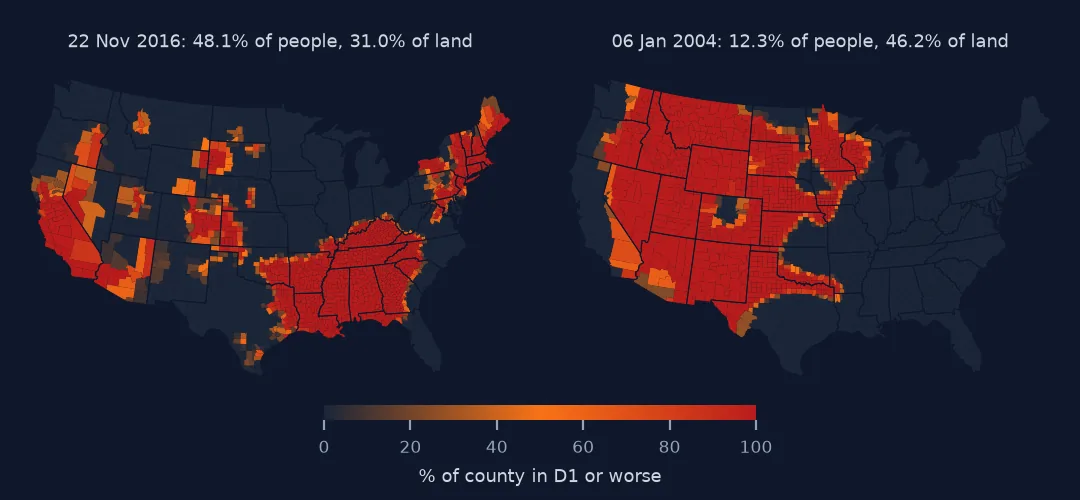
2016-11-22 48.1 31.0
2016-12-27 41.1 24.0
2016-11-29 48.0 31.3
% of people % of land
MapDate
2004-01-06 12.3 46.2
2003-09-16 16.7 50.5
2003-12-30 12.3 46.1
The two extremes show why. In late November 2016 48.1% of people but 31.0% of land were in drought — a drought across the South-East and California's still-lingering one, covering cities. In January 2004 it was the reverse: 46.2% of land and 12.3% of people, with the drought on the High Plains and in the Interior West.
Example 2: people-weeks by state
pw = d.groupby("State").people_d1.sum() / d.MapDate.nunique() / 1e6
print("average people in D1 or worse, millions:", pw.sort_values(ascending=False).head(6).round(2).to_dict())
average people in D1 or worse, millions: {'CA': 17.73, 'TX': 10.65, 'AZ': 4.42, 'FL': 4.3, 'GA': 3.45, 'NC': 2.33}
Averaged over all weeks, California alone accounts for 17.73 million people in drought, Texas for 10.65 million — together more than all other states in the top six combined. A national population share follows California's rainfall more than any other single state's.
Exposure is not impact
Population-weighted drought is an exposure measure: how many people live where the map shows drought. It is the right number for questions about public water supply, wildfire smoke or heat stress, and the wrong one for crop losses, which follow farmland, or for hydropower, which follows rivers. The Drought Monitor publishes area- and population-weighted shares side by side for exactly that reason, and also by agricultural commodity.
City dwellers are often served by water systems that draw on distant reservoirs, so a city in D2 may face no restrictions while a rural well a few miles away runs dry. Exposure figures say where drought is, not who suffers from it.
Details that move the numbers
- Population year. Using 2024 estimates for all 26 years ignores growth in the South and West; for a historical series, join each year's own estimates.
- Connecticut. Since 2022 the Census Bureau reports Connecticut by planning region rather than county, and the Drought Monitor follows it. Mixing older county files with newer statistics leaves Connecticut unmatched.
- Alaska, Hawaii and Puerto Rico. The national population statistics used for comparison are for the contiguous states; keep both sides on the same area.
- Cumulative columns. Use
D1, notD1 + D2 + …, for "D1 or worse"; see drought percentages over 100%.
Internal links
- How to analyse US Drought Monitor county statistics — the county series
- Drought percentages that add up to more than 100% — why D1 means D1 or worse here
- How to measure how many people live near a bike-share station — population exposure with finer units
FAQ
Is the share of people in drought lower than the share of land?
Usually: in 80% of weeks from 2000 to 2025. It is higher when drought reaches the populous coasts, as in November 2016.
Do I need population grids, or are counties enough?
For national weekly shares, counties are within 1.2 points of the Drought Monitor's own figures nine weeks out of ten. For a single large county or a city, use tracts or a grid.