How to download and map an earthquake catalogue in Python

On this page

Problem statement

The USGS earthquake service will hand you a catalogue in one request, which makes it easy to get a file and hard to notice its edges. The service caps a query at 20,000 events and returns the most recent ones when the cap is hit — silently, so a 25-year request can come back as a 10-year catalogue. Magnitudes arrive on several scales, depths include fixed defaults, and the geometry is a point per event that still needs a CRS choice before anything is measured.

Getting the download right is most of this guide: paging past the cap, keeping the fields that matter, and turning the result into a GeoDataFrame that can be counted per area without projecting a spherical mess.

Quick answer

Request in chunks that stay under the cap, then concatenate:

import pandas as pd, requests, geopandas as gpd

API = "https://earthquake.usgs.gov/fdsnws/event/1/query"

def fetch(bbox, start, end, minmag=2.5):
    r = requests.get(API, params={"format": "geojson", "starttime": start, "endtime": end,
                                  "minlongitude": bbox[0], "minlatitude": bbox[1],
                                  "maxlongitude": bbox[2], "maxlatitude": bbox[3],
                                  "minmagnitude": minmag, "orderby": "time-asc",
                                  "limit": 20000}, timeout=180)
    r.raise_for_status()
    f = r.json()["features"]
    if len(f) == 20000:
        raise RuntimeError("hit the 20,000-event cap: split the time range")
    return pd.DataFrame([{
        "id": x["id"], "time": pd.to_datetime(x["properties"]["time"], unit="ms", utc=True),
        "mag": x["properties"]["mag"], "magtype": x["properties"]["magType"],
        "depth_km": x["geometry"]["coordinates"][2],
        "lon": x["geometry"]["coordinates"][0], "lat": x["geometry"]["coordinates"][1],
        "place": x["properties"]["place"]} for x in f])

def fetch_years(bbox, years, minmag=2.5):
    parts = [fetch(bbox, f"{y}-01-01", f"{y}-12-31T23:59:59", minmag) for y in years]
    return pd.concat(parts, ignore_index=True)

BOX = [-122.5, 35.5, -117.5, 38.5]                    # central California
eq = fetch_years(BOX, range(2015, 2025), minmag=2.0)
print(f"{len(eq):,} events, {eq.time.min().date()} to {eq.time.max().date()}, "
      f"M{eq.mag.min():.1f}–{eq.mag.max():.1f}")

18,871 events, 2015-01-01 to 2024-12-31, M2.0–7.1

Year-by-year requests keep every chunk well under the cap and make the failure explicit if one year ever exceeds it.

Map of central California with earthquake epicentres from 2015 to 2024, sized by magnitude. Most events line up along the San Andreas fault and in clusters to the east; a dense red cluster in the south-east corner is the 2019 Ridgecrest sequence. — The catalogue from the code above, re-downloaded for this map: 18,874 events of M2 and above in the guide’s box, 2015–2024. An earlier download of the same query had 18,875 and the latest run above 18,871: ComCat revises events, which is why step 6 says to record the download date. Circles are sized by magnitude. The dense red cluster in the south-east corner is 2019’s Ridgecrest sequence, 5,772 events in one year, and the M7.1 at its centre is the largest event in the catalogue.

The cap is the only part of this that bites, and it bites silently.

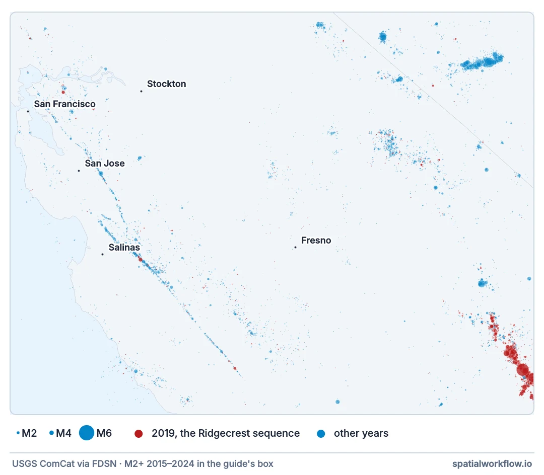
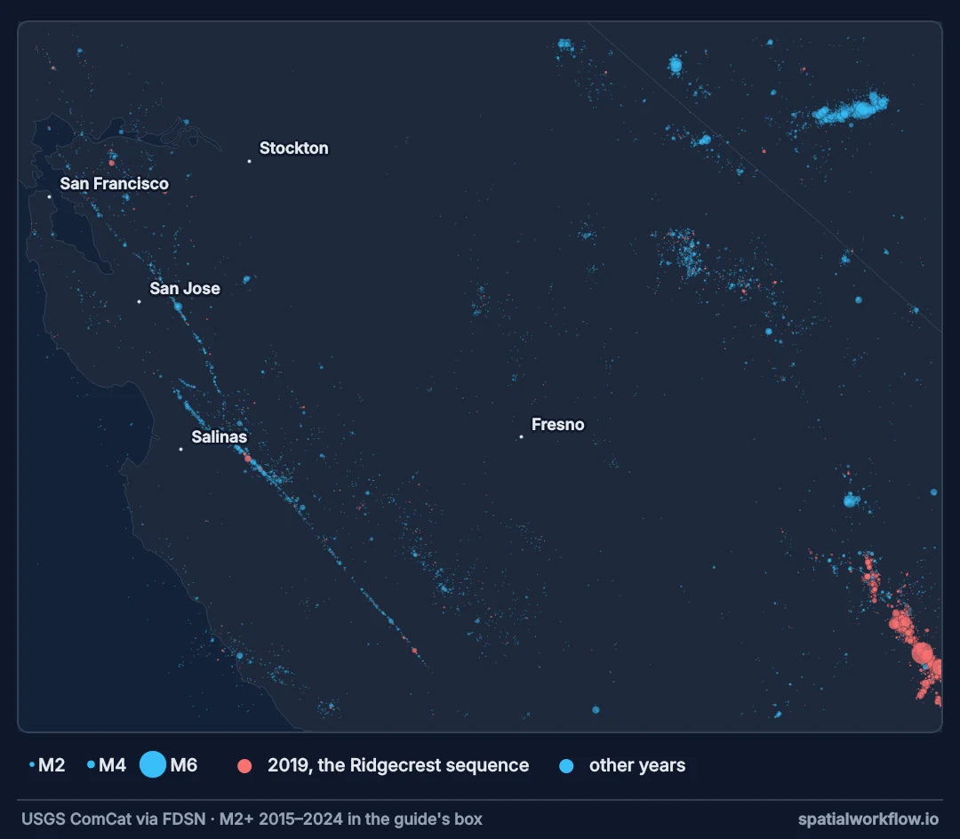
Box, period, magnitude, then page past the cap

1. Choose the box, the period and the minimum magnitude

These three decide how many events come back. A dense network plus a low magnitude threshold plus a decade will exceed any cap.

2. Page, and check for the cap

Request per year or per month and raise if a chunk returns exactly the limit. Silently truncated catalogues are the most common error in this workflow.

3. Clean the fields

Keep id to deduplicate, parse the time as UTC, and keep magType so a later analysis can filter by scale.

4. Build geometry in WGS 84, then project for measurement

Points come in as longitude and latitude. Project to an equal-area or local CRS before counting per unit area or computing distances.

5. Deduplicate across chunks

Boundaries between requests can return the same event twice. Drop duplicates on id.

6. Record the query and the date

A catalogue is a snapshot: magnitudes are revised and events are added. Save the parameters and the download date with the file.

Ten years of central California: two of them are one earthquake sequence.

From a query to counts per area

Example 1 — what the cap does

try:                                               # ten years at M1.0 is well over the cap
    fetch(BOX, "2015-01-01", "2024-12-31", minmag=1.0)
except RuntimeError as e:
    print("raised:", e)
per_year = eq.groupby(eq.time.dt.year).size()
print("events per year at M2.0:", per_year.to_dict())

raised: hit the 20,000-event cap: split the time range
events per year at M2.0: {2015: 883, 2016: 966, 2017: 1129, 2018: 766, 2019: 5769, 2020: 4900, 2021: 1752, 2022: 1094, 2023: 882, 2024: 730}

Example 2 — to a GeoDataFrame, and counts per area

eq = eq.drop_duplicates("id")
gdf = gpd.GeoDataFrame(eq, geometry=gpd.points_from_xy(eq.lon, eq.lat), crs=4326)
metric = gdf.to_crs(3310)                                # California Albers, equal area

cell = 25_000                                            # 25 km grid
metric["gx"] = (metric.geometry.x // cell).astype(int)
metric["gy"] = (metric.geometry.y // cell).astype(int)
dens = metric.groupby(["gx", "gy"]).size().rename("events").reset_index()
print(f"{len(dens)} occupied cells of 625 km²; "
      f"busiest {dens.events.max():,} events; median {dens.events.median():.0f}")
print(metric.groupby(metric.mag.round()).size().rename("events").to_string())

212 occupied cells of 625 km²; busiest 3,136 events; median 13
mag
2.0    12334
3.0     5768
4.0      701
5.0       60
6.0        7
7.0        1

Example 3 — the depth defaults

print("central California, M2.0+:")
print("  most common depths (km):", eq.depth_km.round(1).value_counts().head(3).to_dict())
print(f"  at exactly 10.0 km: {(eq.depth_km == 10.0).mean():.1%}   "
      f"negative (above sea level): {(eq.depth_km < 0).sum():,}")

world = fetch([-180, -90, 180, 90], "2015-01-01", "2024-12-31", minmag=5.5)
print(f"worldwide M5.5+, {len(world):,} events:")
print("  most common depths (km):", world.depth_km.round(1).value_counts().head(3).to_dict())
print(f"  at exactly 10.0 km: {(world.depth_km == 10.0).mean():.1%}")

central California, M2.0+:
  most common depths (km): {2.6: 273, 6.8: 268, 5.0: 260}
  at exactly 10.0 km: 0.3%   negative (above sea level): 358
worldwide M5.5+, 4,518 events:
  most common depths (km): {10.0: 1473, 8.0: 92, 35.0: 83}
  at exactly 10.0 km: 32.6%

A dense local network resolves depth well, so central California has no spike. The global catalogue does: nearly a third of worldwide M5.5+ events sit at exactly 10 km, which is the default used when depth cannot be resolved — not a layer of the crust.

Why the result cap matters

Why the cap matters more than it looks

The service does not error when a query exceeds its limit; it returns the most recent 20,000 events. The result is a valid-looking catalogue whose start date is wrong, and every rate computed from it is wrong in the same direction. Splitting the request by year makes each chunk small and makes the failure loud.

Why an equal-area CRS is needed for density

Counting events per cell in degrees gives cells that shrink towards the poles, so a density map in WGS 84 has a built-in latitude gradient. Projecting to an equal-area CRS — California Albers here — makes every cell the same size on the ground.

Why to keep the event ID

Catalogues are revised. Keeping id lets you deduplicate across overlapping requests, join to later downloads, and fetch the event's own page for products such as ShakeMap.

Where the network cannot resolve depth, the software writes a default — and it shows.

Other services, revised magnitudes and rate limits

Other services: the same FDSN interface is offered by EMSC, GeoNet, INGV and others with the same parameters.
orderby=time-asc makes chunk boundaries predictable.
Time zones: times are UTC; local-day analyses must convert.
Revised magnitudes mean two downloads of the same period can differ.
includedeleted returns events withdrawn from the catalogue.
Rate limits: be polite with a delay between chunked requests.

Internal links

Earthquake catalogues explained — what the fields mean
How to estimate b-value and completeness in Python — the standard analysis
Earthquake counts rise over time in the catalogue — reading trends correctly
How to read a USGS ShakeMap and find who was shaken — from an event to intensity
How to paginate a large feature API in Python — paging in general
How to aggregate points into H3 hexagons and map them — density maps

FAQ

How do I download earthquakes in Python?

Query the USGS FDSN event service for GeoJSON, in chunks small enough to stay under its 20,000-event cap.

Why does my catalogue start later than I asked?

The query hit the cap and the service returned only the most recent events.

What CRS should I use?

Read as WGS 84, then project to an equal-area CRS before density or distance work.

Why are so many events at exactly 10 km depth?

It is a default used when depth cannot be resolved.

Can I get events from outside the US?

Yes — the service is global, and other agencies offer the same FDSN interface.

How do I avoid duplicates between chunks?

Deduplicate on the event id.