The Gutenberg-Richter Law Explained

Problem statement

Small earthquakes are common and large ones rare, and in 1944 Beno Gutenberg and Charles Richter showed that the relationship is remarkably regular: the logarithm of the number of earthquakes at or above a magnitude falls on a straight line, log10 N = a − bM. With b close to 1, each step of one magnitude unit up brings ten times fewer earthquakes. The law is the starting point for every recurrence estimate and hazard model, and it has a consequence that surprises people: although small earthquakes vastly outnumber large ones, almost all the energy is released by the few largest.

This page tests the law on 25 years of the world's M5.5+ earthquakes from the USGS catalogue, estimates a and b, compares the counts it predicts with those observed up to magnitude 9, measures how the seismic moment is shared between small and large events, and compares b for shallow and deep earthquakes.

Quick answer

Count earthquakes per magnitude unit and fit b by maximum likelihood above a complete threshold:

m = ev.mag.round(1)
b = np.log10(np.e) / (m.mean() - (5.5 - 0.05))
for lo, hi in ((5.5, 6.5), (6.5, 7.5), (7.5, 8.5), (8.5, 9.5)):
    print(f"M{lo}-{hi}: {((m >= lo) & (m < hi)).sum():>6,} earthquakes")
print(f"b = {b:.3f} from {len(m):,} earthquakes of M5.5 and above, 2000-2024")

M5.5-6.5: 11,193 earthquakes
M6.5-7.5:  1,009 earthquakes
M7.5-8.5:    127 earthquakes
M8.5-9.5:      5 earthquakes
b = 1.028 from 12,334 earthquakes of M5.5 and above, 2000-2024

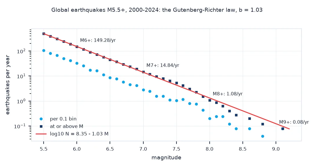
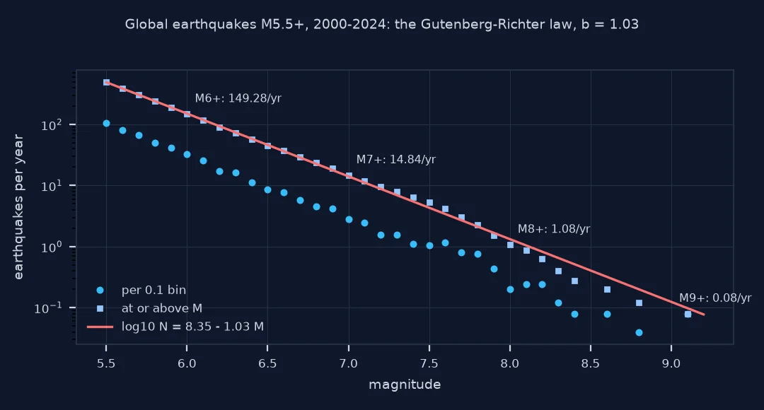
Each magnitude unit up holds about ten times fewer earthquakes: 11,193 between M5.5 and M6.5, 1,009 up to M7.5, 127 up to M8.5 and 5 above. The maximum-likelihood b-value is 1.028.

What a and b predict, who releases the energy, depth

1. What a and b predict

The a-value sets the level, the b-value the slope. Predict the yearly number at or above each magnitude and compare with the catalogue:

years = 25
a = np.log10(len(m) / years) + b * 5.5
for mag in (6, 7, 8, 9):
    pred = 10 ** (a - b * mag)
    obs = (m >= mag).sum() / years
    print(f"M{mag}+: predicted {pred:7.2f} a year, observed {obs:7.2f} a year")
print(f"a = {a:.2f} (yearly, M0 and above, extrapolated)")

M6+: predicted  151.02 a year, observed  149.28 a year
M7+: predicted   14.15 a year, observed   14.84 a year
M8+: predicted    1.33 a year, observed    1.08 a year
M9+: predicted    0.12 a year, observed    0.08 a year
a = 8.35 (yearly, M0 and above, extrapolated)

With a = 8.35 and b = 1.028, the law predicts 151 earthquakes of M6 or more a year, against 149 observed, and 14.2 of M7 or more, against 14.8. At the top end it predicts 1.33 of M8+ a year against 1.08 observed, and one M9+ every eight years, against two in 25 years: close, given how few great earthquakes there are.

2. Who releases the energy

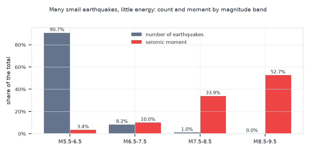
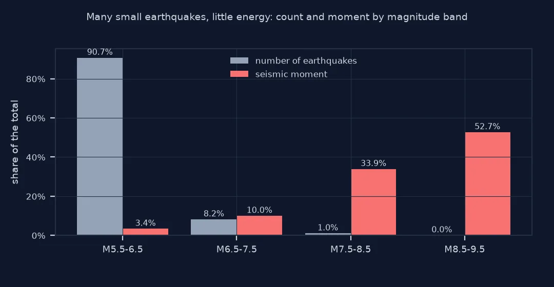
Seismic moment grows by a factor of 10^1.5, about 32, per magnitude unit, faster than the number of earthquakes falls. Share the total moment by magnitude band:

m0 = 10 ** (1.5 * ev.mag + 9.1)
bands = pd.cut(ev.mag, [5.5, 6.5, 7.5, 8.5, 9.5], right=False)
share = m0.groupby(bands, observed=True).sum() / m0.sum()
print((share * 100).round(1).rename("% of moment").to_string())
top = ev.assign(m0=m0).nlargest(3, "m0")
print(f"three largest earthquakes: {top.m0.sum() / m0.sum():.0%} of the moment of all {len(ev):,}")
print(top[["time", "mag", "place"]].assign(time=top.time.str[:10]).to_string(index=False))

mag
[5.5, 6.5)     3.4
[6.5, 7.5)    10.0
[7.5, 8.5)    33.9
[8.5, 9.5)    52.7
three largest earthquakes: 46% of the moment of all 12,334
      time  mag                                     place
2004-12-26  9.1 2004 Sumatra - Andaman Islands Earthquake
2011-03-11  9.1       2011 Great Tohoku Earthquake, Japan
2010-02-27  8.8              2010 Maule, Chile Earthquake

The 11,193 earthquakes between M5.5 and M6.5, 91% of the catalogue, released 3.4% of its moment; the 5 of M8.5 and above released 52.7%. The three largest alone, Sumatra 2004, Tohoku 2011 and Maule 2010, account for 46% of the moment of all 12,334.

3. Shallow and deep earthquakes

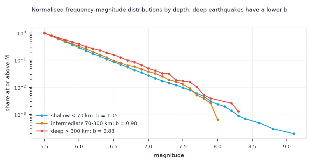
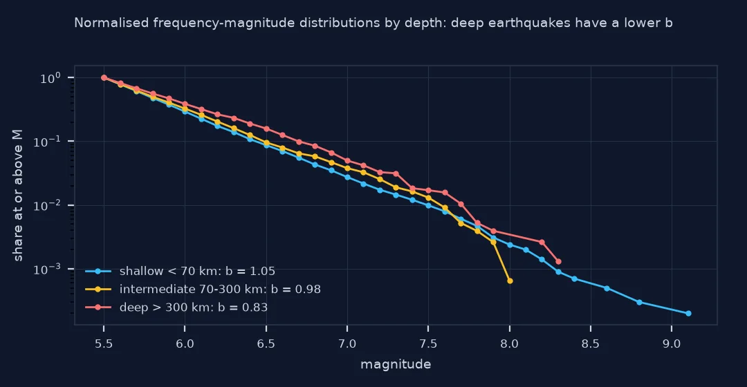
The b-value is not universal. Compare earthquakes shallower than 70 km with intermediate and deep ones:

for name, sel in (("shallow (< 70 km)", ev.depth < 70), ("intermediate (70-300 km)", ev.depth.between(70, 300)), ("deep (> 300 km)", ev.depth > 300)):
    mm = m[sel]
    bb = np.log10(np.e) / (mm.mean() - 5.45)
    se = bb / np.sqrt(len(mm))
    print(f"{name:>25}: {len(mm):>5,} earthquakes, b = {bb:.2f} ± {se:.2f}")

        shallow (< 70 km): 10,039 earthquakes, b = 1.05 ± 0.01
 intermediate (70-300 km): 1,532 earthquakes, b = 0.98 ± 0.03
          deep (> 300 km):   763 earthquakes, b = 0.83 ± 0.03

Shallow earthquakes have b = 1.05 ± 0.01 and intermediate-depth ones 0.98 ± 0.03, but deep earthquakes, below 300 km, have 0.83 ± 0.03: proportionally more large events, a difference well outside the uncertainties.

Is magnitude 5.5 really complete

The data used on this page

Every earthquake of magnitude 5.5 or more worldwide from 2000 to 2024 in the USGS ComCat catalogue, from the FDSN event service. At M5.5 the global catalogue is taken to be complete for this period.

from pathlib import Path

import numpy as np
import pandas as pd
import requests

Path("data").mkdir(exist_ok=True)
p = Path("data/global_m55_2000_2024.csv")
if not p.exists():
    r = requests.get("https://earthquake.usgs.gov/fdsnws/event/1/query", timeout=600,
                     params=dict(format="csv", starttime="2000-01-01", endtime="2025-01-01", minmagnitude=5.5, orderby="time-asc"))
    r.raise_for_status()
    p.write_bytes(r.content)
ev = pd.read_csv(p)
ev = ev[ev["type"] == "earthquake"].reset_index(drop=True)
print(f"{len(ev):,} earthquakes; M{ev.mag.min()} to M{ev.mag.max()}; magnitude types {ev.magType.value_counts().head(4).to_dict()}")

12,334 earthquakes; M5.5 to M9.1; magnitude types {'mww': 5312, 'mwc': 4132, 'mwb': 1934, 'mb': 776}

The catalogue holds 12,334 earthquakes from M5.5 to M9.1. Nearly all have moment magnitudes of one kind or another (Mww, Mwc, Mwb); 776 have body-wave magnitudes (mb).

Example 1: is M5.5 really complete?

Check the frequency-magnitude distribution just above the threshold: in a complete catalogue the counts per 0.1 bin fall steadily from the first bin:

c = m.value_counts().sort_index().loc[5.5:6.2]
print(c.to_string())
print(f"ratio of successive bins: {(c.values[1:] / c.values[:-1]).round(2).tolist()}; expected for b = {b:.2f}: {10 ** (-b * 0.1):.2f}")

mag
5.5    2633
5.6    2034
5.7    1662
5.8    1240
5.9    1033
6.0     824
6.1     647
6.2     435
ratio of successive bins: [0.77, 0.82, 0.75, 0.83, 0.8, 0.79, 0.67]; expected for b = 1.03: 0.79

From the threshold up, each 0.1 bin holds between 67% and 83% of the one before, scattered around the 79% that b = 1.03 implies. There is no deficit in the first bins, which is what an incomplete catalogue would show; M5.5 is complete here.

Magnitudes follow an exponential distribution

The Gutenberg-Richter law says magnitudes above a threshold follow an exponential distribution, which is why a single parameter, b, describes the shape and why the maximum-likelihood estimate is a simple function of the mean magnitude. Why nature produces it is still debated: it is what many systems close to failure produce, where a slip of any size can trigger more, with no preferred scale. Values of b near 1 are found from small regions to the whole globe; departures, higher in volcanic areas and swarms, lower in some highly stressed zones, are among the most studied signals in seismology.

The energy consequence follows from the logarithms. Each magnitude unit brings about 10 times fewer earthquakes but about 32 times more moment per earthquake, so each unit up contributes about 3 times more moment in total. The largest earthquakes therefore dominate any sum of energy, and a quarter-century of global seismicity is, in moment, mostly a handful of great earthquakes. That is also why the law cannot run upwards forever: fault size limits the largest possible earthquake, and somewhere above magnitude 9 the line must bend.

Completeness, moment and short records

• Completeness: fit only above the magnitude of completeness; see the b-value fix.
• Magnitude types: global catalogues mix body-wave (mb) and moment magnitudes; mb saturates around 6 to 6.5, which can bend the distribution.
• Moment from magnitude: M0 = 10^(1.5M + 9.1) N m is exact only for moment magnitude.
• Short records: 25 years contains two M9 earthquakes, too few to test the law at the top end.

Internal links

• How to estimate b-value and completeness in Python
• How to estimate the probability of an earthquake from a catalogue in Python — the law used for forecasting
• Earthquake catalogues explained: magnitudes, completeness and declustering — what a catalogue holds

FAQ

What is the Gutenberg-Richter law?

The empirical relation log10 N = a − bM between magnitude M and the number N of earthquakes at or above it; b is usually close to 1.

What does the b-value mean?

The slope of the relation: with b = 1, every unit increase in magnitude brings ten times fewer earthquakes.

Do small earthquakes release pressure and prevent big ones?

No: because moment grows about 32 times per magnitude unit while numbers fall only about 10 times, small earthquakes release a tiny fraction of the energy. In 2000–2024, the 11,193 earthquakes between M5.5 and M6.5 released 3.4% of the moment of all M5.5+ earthquakes; the five of M8.5 and above, 52.7%.

How many great earthquakes does the law predict?

Fitted to the world's M5.5+ earthquakes of 2000–2024, it predicts 1.33 earthquakes of M8 or more a year (1.08 were observed) and 0.12 of M9 or more, one every eight years; two happened in the 25 years.