
How to Map Hail Reports by County: Sizes, Counts and the One-Inch Spike
On this page
Problem statement
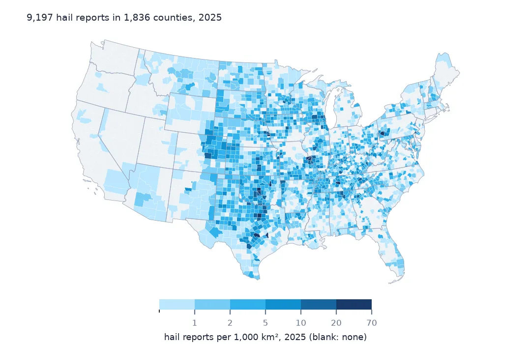
Hail is the second most common event in the Storm Events database, with 9,205 reports in 2025, and every one is tied to a county. Mapping them is easy. The harder part is reading the map: the densest hail counties are the ones with the most people watching, sizes cluster on the coins and balls that observers compare stones to, and a county's count depends on its area. This page maps 2025's hail reports by county, shows the one-inch spike in the size distribution, and normalises by area and population so the map shows where hail fell rather than where people were.
Quick answer
Hail rows are all county-based (CZ_TYPE == "C"), so STATE_FIPS zero-padded to two digits plus CZ_FIPS padded to three is the county GEOID. Count reports per GEOID, merge onto Census county boundaries, and divide by area before colouring the map.
hail = ev[ev.EVENT_TYPE == "Hail"].copy()
hail["GEOID"] = hail.STATE_FIPS.astype(int).astype(str).str.zfill(2) + hail.CZ_FIPS.astype(int).astype(str).str.zfill(3)
per = hail.groupby("GEOID").agg(reports=("EVENT_ID", "size"), largest_in=("MAGNITUDE", "max"))
m = counties.merge(per, on="GEOID", how="left").fillna({"reports": 0})
print(f"{len(hail):,} hail reports in {(m.reports > 0).sum():,} of {len(m):,} counties; matched {hail.GEOID.isin(counties.GEOID).mean():.1%}")
9,205 hail reports in 1,836 of 3,222 counties; matched 99.9%
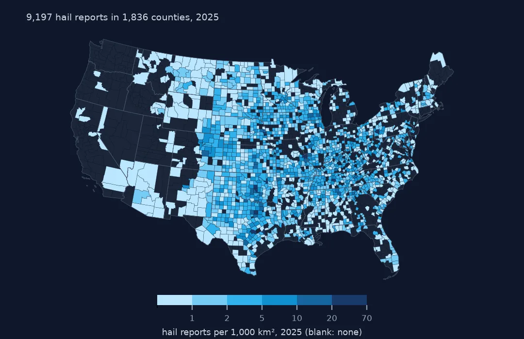
9,205 reports fell in 1,836 of the 3,222 counties and county-equivalents, and 99.9% of reports match a county GEOID. The few that miss are in Connecticut, whose counties were replaced by planning regions in the 2023 boundaries, and in Puerto Rico and Alaska, where the reports name places the generalised county file does not carry.
Counting, sizing and normalising hail
1. Hail is reported by county
print(hail.CZ_TYPE.value_counts().to_dict(), "| magnitude type:", hail.MAGNITUDE_TYPE.value_counts(dropna=False).to_dict())
print(f"hail size in inches: median {hail.MAGNITUDE.median():.2f}, largest {hail.MAGNITUDE.max():.2f}")
{'C': 9205} | magnitude type: {nan: 9205}
hail size in inches: median 1.00, largest 6.00
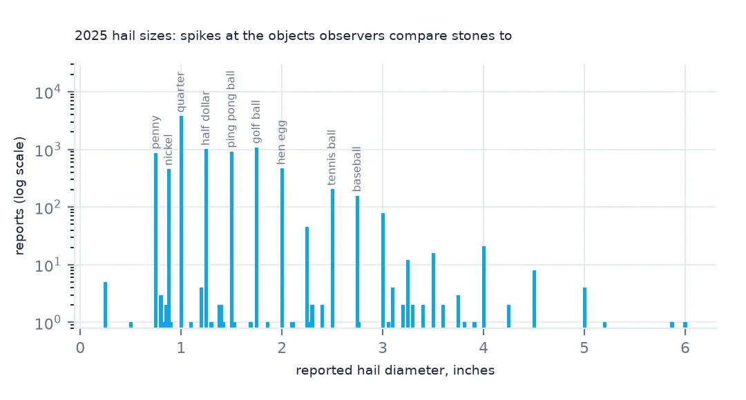
Every hail row is county-based and MAGNITUDE holds the stone diameter in inches (MAGNITUDE_TYPE, which records how wind was measured, is blank for hail). The median report is 1.00 inch and the largest 6.00 inches.
2. Sizes cluster on familiar objects
sizes = hail.MAGNITUDE.value_counts().sort_index()
print(sizes[sizes >= 100].to_string())
print(f"reports at exactly 1.00 inch: {(hail.MAGNITUDE == 1).mean():.1%}; at 0.95-0.99 or 1.01-1.05: "
      f"{hail.MAGNITUDE.between(0.95, 1.05).sum() - (hail.MAGNITUDE == 1).sum()}")
MAGNITUDE
0.75 872
0.88 454
1.00 3784
1.25 1012
1.50 919
1.75 1090
2.00 468
2.50 204
2.75 158
reports at exactly 1.00 inch: 41.1%; at 0.95-0.99 or 1.01-1.05: 0
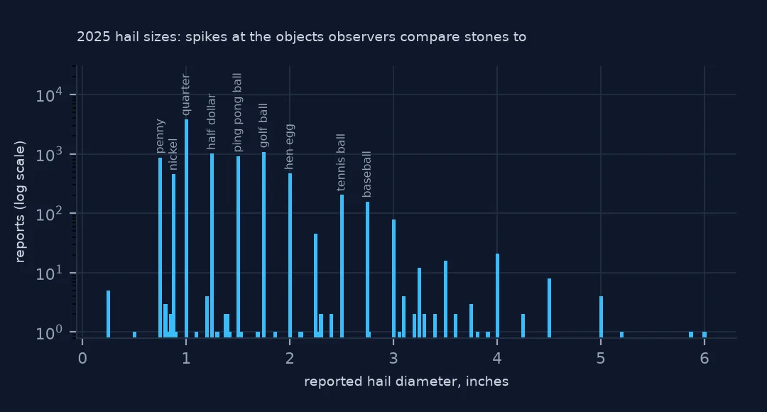
The sizes are not continuous. 41.1% of reports are exactly 1.00 inch, the size of a quarter and the National Weather Service's severe threshold, and none fall between 0.95 and 1.05 apart from it. The other peaks are objects too: 0.75 (a penny), 0.88 (a nickel), 1.75 (a golf ball) and 2.75 (a baseball). Observers compare stones to a size chart and report the object, so a histogram with fine bins shows the chart, not the hail. Bin into classes such as under 1 inch, 1–2 inches and 2 inches or more.
3. Normalise by area
m["area_km2"] = m.area / 1e6
m["per_1000km2"] = m.reports / m.area_km2 * 1000
top = m.sort_values("reports", ascending=False).head(5)[["NAMELSAD", "STUSPS", "reports", "area_km2", "per_1000km2"]]
print(top.round(1).to_string(index=False))
print(m.sort_values("per_1000km2", ascending=False).head(5)[["NAMELSAD", "STUSPS", "reports", "per_1000km2"]].round(1).to_string(index=False))
NAMELSAD STUSPS reports area_km2 per_1000km2
St. Louis County MO 93.0 1350.2 68.9
El Paso County CO 92.0 5511.1 16.7
Oklahoma County OK 87.0 1860.1 46.8
Tulsa County OK 82.0 1539.7 53.3
Williamson County TX 73.0 2926.2 24.9
NAMELSAD STUSPS reports per_1000km2
St. Louis County MO 93.0 68.9
St. Louis city MO 11.0 66.8
Tulsa County OK 82.0 53.3
Cleveland County OK 71.0 49.8
Harrisonburg city VA 2.0 48.1
St. Louis County, Missouri tops both lists, with 93 reports and 68.9 per 1,000 km². St. Louis city, an independent city with its own GEOID, comes second by density on just 11 reports. El Paso County, Colorado (Colorado Springs) has nearly as many reports (92) but is four times larger. Every county high on the density list contains a city.
4. Population drives reports
pop = pd.read_csv("https://www2.census.gov/programs-surveys/popest/datasets/2020-2024/counties/totals/co-est2024-alldata.csv",
                  encoding="latin-1", dtype={"STATE": str, "COUNTY": str}, usecols=["STATE", "COUNTY", "POPESTIMATE2024"])
m = m.merge(pop.assign(GEOID=pop.STATE + pop.COUNTY)[["GEOID", "POPESTIMATE2024"]], on="GEOID", how="left")
plains = m[m.STUSPS.isin(["KS", "NE", "OK", "TX", "SD", "CO"])]
print(f"Plains counties: Spearman rank correlation of reports per 1000 km2 with people per km2: "
      f"{plains.per_1000km2.corr(plains.POPESTIMATE2024 / plains.area_km2, method='spearman'):.2f}")
Plains counties: Spearman rank correlation of reports per 1000 km2 with people per km2: 0.25
Across six Plains states, reports per 1,000 km² rise with population density, with a rank correlation of 0.25. That is weak but positive. Hail falls on empty rangeland as often as on suburbs, but nobody reports it there. A per-area map therefore partly maps people. Counting hail days per county, or using radar-derived hail estimates, reduces that bias.
Large hail and hail damage
The data used on this page
The National Centers for Environmental Information's Storm Events Database details file for 2025, Census Bureau 2023 county boundaries and 2024 county population estimates.
from pathlib import Path

import geopandas as gpd
import numpy as np
import pandas as pd
import requests

Path("data").mkdir(exist_ok=True)
# NOAA NCEI Storm Events Database: the 2025 details and fatalities files (revision c20260819) and the 2024 details file
# (revision c20260728), saved on this site on 15 October 2026 because NCEI replaces a year's files whenever it revises
# them and the old names disappear. Live: https://www.ncei.noaa.gov/pub/data/swdi/stormevents/csvfiles/
FILES = ["storm-events-details-2025-c20260819.csv.gz", "storm-events-fatalities-2025-c20260819.csv.gz",
         "storm-events-details-2024-c20260728.csv.gz"]
for name in FILES:
    if not Path(f"data/{name}").exists():
        Path(f"data/{name}").write_bytes(requests.get(f"https://data.spatialworkflow.io/{name}", timeout=600).content)
ev = pd.read_csv("data/storm-events-details-2025-c20260819.csv.gz", low_memory=False)


def dollars(s):
    """Damage is stored as text: '10.00K', '1.60B', '0' or blank. A blank means no estimate, not zero."""
    s = s.str.strip()
    return pd.to_numeric(s.str.rstrip("KMB"), errors="coerce") * s.str[-1].map({"K": 1e3, "M": 1e6, "B": 1e9}).fillna(1.0)


def times(df):
    """Event times are local to the county or zone ('CST-6'), with a two-digit year."""
    df["begin"] = pd.to_datetime(df.BEGIN_DATE_TIME, format="%d-%b-%y %H:%M:%S")
    df["end"] = pd.to_datetime(df.END_DATE_TIME, format="%d-%b-%y %H:%M:%S")
    df["utc_offset"] = df.CZ_TIMEZONE.str.extract(r"(-?\d+)$")[0].astype(int)
    df["begin_utc"] = df.begin - pd.to_timedelta(df.utc_offset, unit="h")
    df["prop"], df["crops"] = dollars(df.DAMAGE_PROPERTY), dollars(df.DAMAGE_CROPS)
    return df


ev = times(ev)
for name, url in {"cb_2023_us_county_20m.zip": "https://www2.census.gov/geo/tiger/GENZ2023/shp/cb_2023_us_county_20m.zip",
                  "cb_2023_us_state_20m.zip": "https://www2.census.gov/geo/tiger/GENZ2023/shp/cb_2023_us_state_20m.zip"}.items():
    if not Path(f"data/{name}").exists():
        Path(f"data/{name}").write_bytes(requests.get(url, timeout=300).content)
counties = gpd.read_file("data/cb_2023_us_county_20m.zip").to_crs(5070)
states = gpd.read_file("data/cb_2023_us_state_20m.zip").to_crs(5070)
print(f"{len(ev):,} Storm Events records for 2025, {ev.EPISODE_ID.nunique():,} episodes, {ev.EVENT_TYPE.nunique()} event types")
72,360 Storm Events records for 2025, 9,846 episodes, 48 event types
Example 1: significant hail
big = hail[hail.MAGNITUDE >= 2]
print(f"hail of 2 inches or more: {len(big):,} reports ({len(big) / len(hail):.1%}) in {big.GEOID.nunique()} counties")
print(big.groupby("STATE").size().sort_values(ascending=False).head(5).to_dict())
print(hail.sort_values("MAGNITUDE", ascending=False)[["STATE", "CZ_NAME", "begin", "MAGNITUDE"]].head(3).to_string(index=False))
hail of 2 inches or more: 1,046 reports (11.4%) in 483 counties
{'TEXAS': 248, 'OKLAHOMA': 91, 'COLORADO': 82, 'KANSAS': 77, 'NEBRASKA': 76}
STATE CZ_NAME begin MAGNITUDE
TEXAS DICKENS 2025-05-25 15:33:00 6.00
TEXAS MENARD 2025-05-26 15:23:00 5.87
TEXAS FLOYD 2025-04-24 17:29:00 5.20
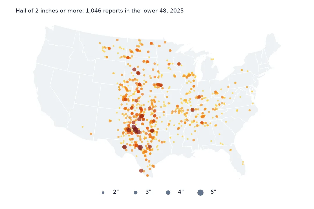
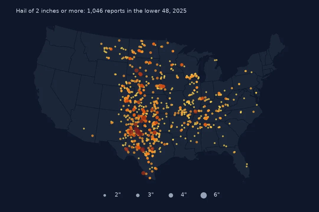
1,046 reports (11.4%) were 2 inches or more, the Storm Prediction Center's threshold for significant hail, in 483 counties. Texas had 248 of them, ahead of Oklahoma (91) and Colorado (82). The three largest stones were all in West Texas: 6.00 inches in Dickens County on 25 May, 5.87 in Menard County the next day and 5.20 in Floyd County in April. Large-hail maps lean further toward the High Plains than the all-sizes map does.
Example 2: hail damage
print(f"hail reports with a property estimate: {hail.prop.notna().mean():.1%}; of those zero: {(hail.prop == 0).mean() / hail.prop.notna().mean():.1%}; "
      f"total ${hail.prop.sum() / 1e6:,.1f} million")
hail reports with a property estimate: 66.4%; of those zero: 92.7%; total $60.1 million
Only 66.4% of hail reports carry a property damage estimate, and 92.7% of those are zero. Hail damage adds up to only $60.1 million in the file, far below insurers' hail losses, because offices rarely have the claims data. Use hail reports to map where hail fell, and do not use them to estimate its cost.
Why hail reports follow people
A hail report needs someone to see the hail, measure or compare it, and tell the Weather Service, by phone, through a spotter network or on social media. Offices also look for reports to confirm their warnings, and they look hardest where warnings cover towns. The result is a map with three layers: the climatology of hail (most frequent on the High Plains from Texas to South Dakota), population (cities collect reports), and office practice (some offices chase reports more than others).
None of this makes the data wrong. It describes what was observed. But a map of reports per county should carry that caveat, and a comparison between an urban and a rural county should be done on hail days or with radar, not raw counts.
County-map details
- Independent cities (St. Louis, Baltimore, the Virginia cities) are their own GEOIDs and small, so they jump to the top of any per-area ranking on a handful of reports.
- Connecticut. Storm Events still uses the eight old counties, and 2023 Census boundaries have nine planning regions. Join Connecticut with older boundaries.
- A colour scale. Report counts are highly skewed, so use quantile or logarithmic classes. A linear scale makes the map almost one colour.
- Zero reports is not zero hail. Leave counties with no reports as missing or the lightest class, and say so in the legend.
Internal links
- How to read the Storm Events database — the files and fields
- Storm Events will not join to counties — why the county key works for hail
- How to chart the severe weather season — when hail falls
FAQ
Why are so many hail reports exactly one inch?
Observers compare hailstones to coins and balls, and a quarter is 1.00 inch, which is also the severe hail threshold. In 2025, 41.1% of reports were exactly 1.00 inch.
How do I join Storm Events hail reports to counties?
Build the GEOID from STATE_FIPS (two digits) and CZ_FIPS (three digits). Hail rows are all county-based, so the key matches Census county boundaries.