Internet Latency Explained: Milliseconds, Distance and Loaded Latency

Problem statement

Speed tests report latency as well as speed: how many milliseconds a small packet takes to reach the test server and come back. For video calls and games it matters more than raw speed. Ookla's tiles carry idle latency and, since 2023, latency measured while downloading and uploading, which is often far higher. This page explains the three figures with the April–June 2026 data: typical values for fixed and mobile networks, how latency relates to speed, how it varies by state, and how much it rises under load.

Quick answer

Idle latency (avg_lat_ms) is the round trip with the line quiet; loaded latency (avg_lat_down_ms, avg_lat_up_ms) is measured while the line is busy. Under 20 ms idle is good for a wired connection. A large rise under load, called bufferbloat, is what makes calls stutter on an otherwise fast line.

print(f"idle latency, tests-weighted median: fixed {wmedian(fixed.avg_lat_ms, fixed.tests):.0f} ms, mobile {wmedian(mobile.avg_lat_ms, mobile.tests):.0f} ms")
ok = fixed.dropna(subset=["avg_lat_down_ms"])
print(f"fixed latency while downloading: {wmedian(ok.avg_lat_down_ms, ok.tests):.0f} ms; while uploading: {wmedian(ok.dropna(subset=['avg_lat_up_ms']).avg_lat_up_ms, ok.dropna(subset=['avg_lat_up_ms']).tests):.0f} ms")

idle latency, tests-weighted median: fixed 12 ms, mobile 27 ms
fixed latency while downloading: 207 ms; while uploading: 159 ms

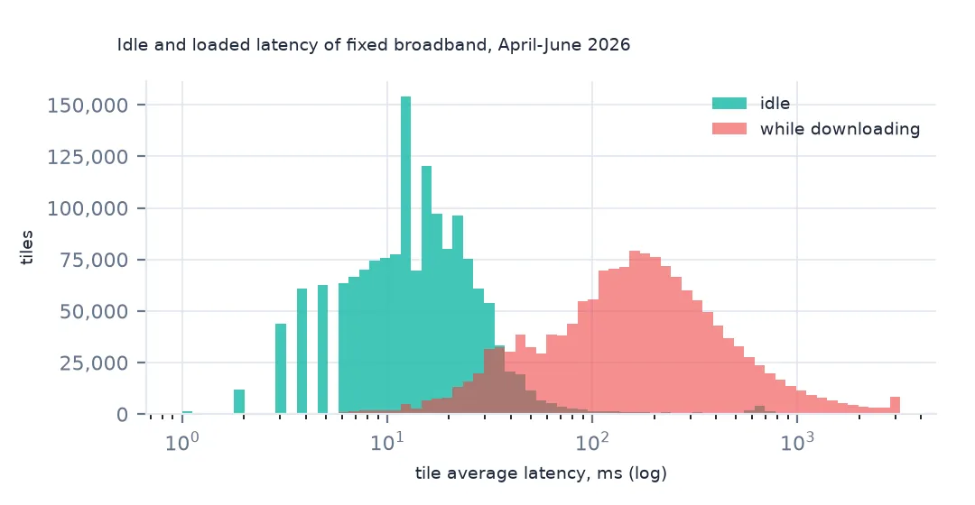
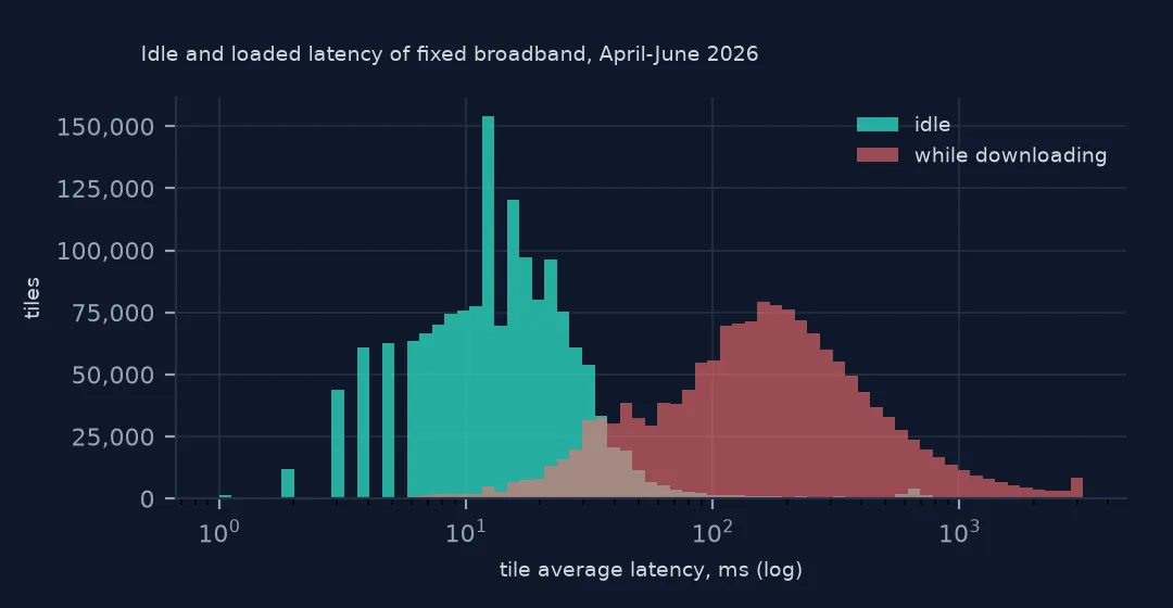
The median fixed-broadband test sees 12 ms of idle latency, and mobile 27 ms. While downloading, fixed latency rises to 207 ms, and while uploading to 159 ms. The connection stays fast, but anything interactive on it waits.

Distribution, speed and states

1. The distribution

print(fixed.avg_lat_ms.describe(percentiles=[0.1, 0.5, 0.9]).loc[["10%", "50%", "90%", "max"]].to_dict())

{'10%': 5.0, '50%': 14.0, '90%': 31.0, 'max': 2656.0}

Across tiles, idle latency runs from 5 ms at the 10th percentile to 31 ms at the 90th, with a long tail to 2,656 ms, satellite links and faulty tests.

2. Latency and speed

print(f"rank correlation of idle latency with download speed across tiles: {fixed.avg_lat_ms.corr(fixed.avg_d_kbps, method='spearman'):.2f}")
q = pd.qcut(fixed.avg_d_kbps, 5, labels=["slowest", "2", "3", "4", "fastest"])
print(fixed.groupby(q, observed=True).avg_lat_ms.median().to_dict())

rank correlation of idle latency with download speed across tiles: -0.33
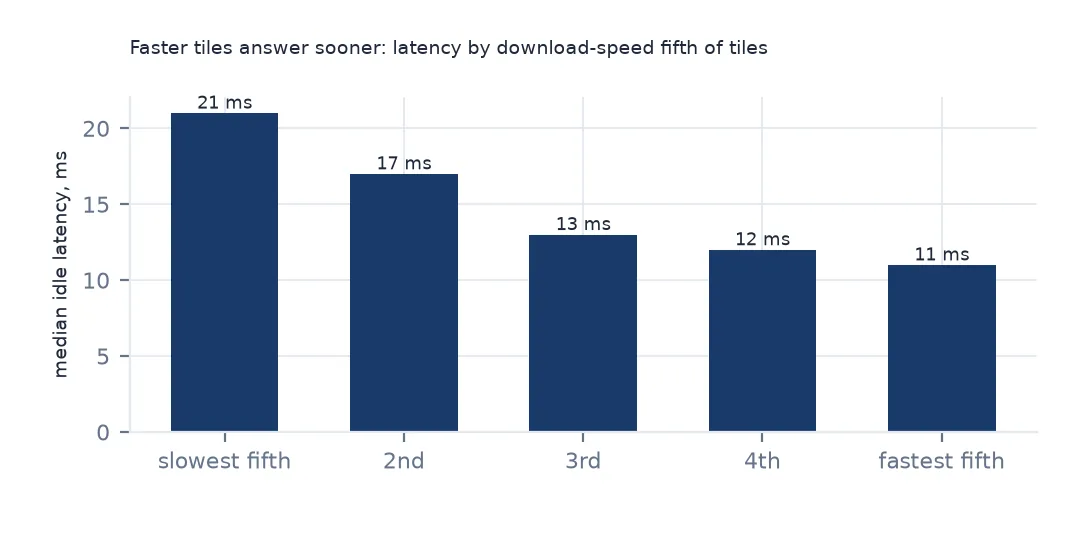
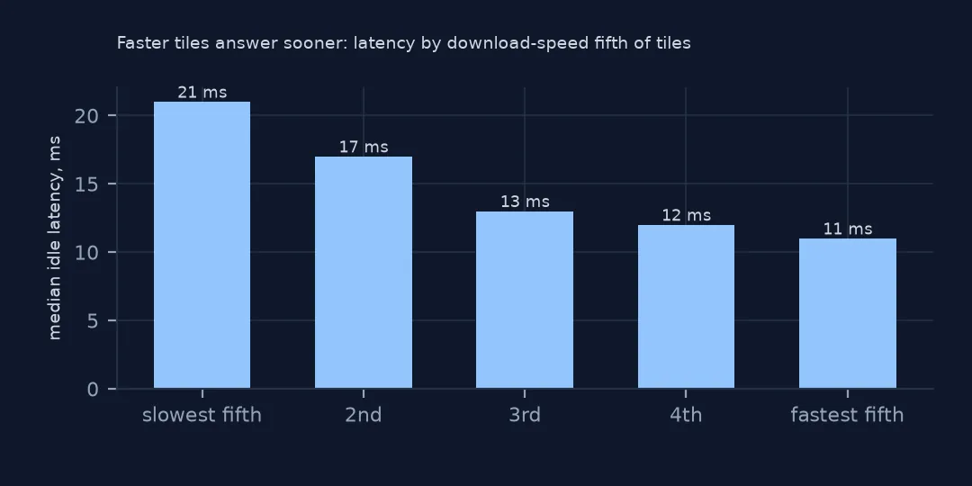
{'slowest': 21.0, '2': 17.0, '3': 13.0, '4': 12.0, 'fastest': 11.0}

Faster tiles have lower latency (rank correlation −0.33): median latency falls from 21 ms in the slowest fifth of tiles to 11 ms in the fastest. Both reflect the access technology, since fibre is fast and quick and DSL and satellite are neither.

3. By state

s = fixed.groupby("STUSPS").apply(lambda d: wmedian(d.avg_lat_ms, d.tests), include_groups=False).sort_values()
print("lowest:", s.head(4).to_dict(), "highest:", s.tail(4).to_dict())

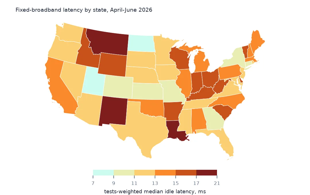
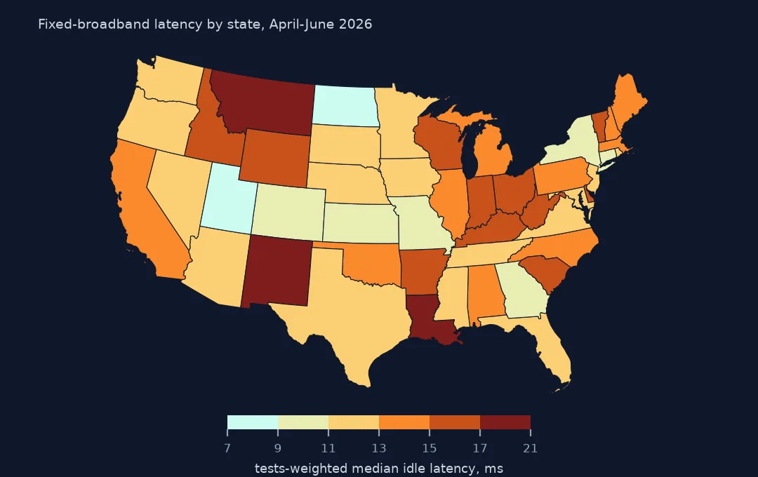
lowest: {'ND': 8, 'UT': 8, 'KS': 9, 'CO': 10} highest: {'SC': 16, 'LA': 17, 'NM': 19, 'MT': 20}

By state, median idle latency is lowest in North Dakota and Utah (8 ms), Kansas and Colorado, and highest in South Carolina, Louisiana, New Mexico and Montana (20 ms). North Dakota's low figure reflects its rural fibre co-operatives, and Montana's high one distance.

Bufferbloat and mobile

The data used on this page

Ookla's Speedtest open data performance tiles for fixed broadband and mobile networks (April–June 2026), read from Amazon S3, and Census Bureau 2023 county boundaries.

from pathlib import Path

import duckdb
import geopandas as gpd
import numpy as np
import pandas as pd
import requests

Path("data").mkdir(exist_ok=True)
# Ookla Speedtest open data (AWS Open Data, keyless): one Parquet file per quarter and network type, zoom-16 web
# Mercator tiles with average speeds, latency, tests and devices. Published quarterly under fixed names.
BASE = "https://ookla-open-data.s3.amazonaws.com/parquet/performance"


def tiles(kind, year, q):
    """One quarter's tiles inside a box around the contiguous US, cached locally as Parquet."""
    path = f"data/ookla-{kind}-{year}q{q}-conus.parquet"
    if not Path(path).exists():
        url = f"{BASE}/type={kind}/year={year}/quarter={q}/{year}-{(q - 1) * 3 + 1:02d}-01_performance_{kind}_tiles.parquet"
        con = duckdb.connect()
        con.sql("INSTALL httpfs; LOAD httpfs;")
        con.sql(f"""COPY (SELECT quadkey, tile_x, tile_y, avg_d_kbps, avg_u_kbps, avg_lat_ms, avg_lat_down_ms, avg_lat_up_ms, tests, devices
                         FROM read_parquet('{url}') WHERE tile_x BETWEEN -125 AND -66 AND tile_y BETWEEN 24 AND 50
                         ORDER BY quadkey) TO '{path}' (FORMAT parquet)""")
    return pd.read_parquet(path)


for name in ["cb_2023_us_county_20m.zip"]:
    if not Path(f"data/{name}").exists():
        Path(f"data/{name}").write_bytes(requests.get(f"https://www2.census.gov/geo/tiger/GENZ2023/shp/{name}", timeout=300).content)
counties = gpd.read_file("data/cb_2023_us_county_20m.zip")
counties = counties[~counties.STUSPS.isin(["AK", "HI", "PR"])].to_crs(4326)


def in_counties(df):
    """Attach the county each tile's centre falls in; tiles outside the lower 48 (Canada, Mexico, sea) drop out."""
    pts = gpd.GeoDataFrame(df, geometry=gpd.points_from_xy(df.tile_x, df.tile_y), crs=4326)
    j = gpd.sjoin(pts, counties[["GEOID", "STUSPS", "NAME", "geometry"]], predicate="within")
    return pd.DataFrame(j.drop(columns=["geometry", "index_right"]))


def wmedian(values, weights):
    """Median of tile averages, each tile counted once per test."""
    o = np.argsort(values.to_numpy())
    v, w = values.to_numpy()[o], weights.to_numpy()[o]
    c = np.cumsum(w)
    return v[np.searchsorted(c, c[-1] / 2)]


fixed = in_counties(tiles("fixed", 2026, 2))
mobile = in_counties(tiles("mobile", 2026, 2))
print(f"Ookla fixed broadband, April-June 2026: {len(fixed):,} tiles in the lower 48, {fixed.tests.sum():,} tests")

Ookla fixed broadband, April-June 2026: 1,548,841 tiles in the lower 48, 15,134,971 tests

Example 1: bufferbloat: the rise under load

ok = ok.assign(rise=ok.avg_lat_down_ms - ok.avg_lat_ms)
print(f"latency rise while downloading: median {ok.rise.median():.0f} ms; tiles where it at least doubles: {(ok.avg_lat_down_ms >= 2 * ok.avg_lat_ms).mean():.1%}")

latency rise while downloading: median 146 ms; tiles where it at least doubles: 93.7%

Latency rises by a median of 146 ms while downloading, and at least doubles in 93.7% of tiles. That is bufferbloat, and it is a property of routers and access networks, not of the advertised speed.

Example 2: mobile latency by state

m = mobile.groupby("STUSPS").apply(lambda d: wmedian(d.avg_lat_ms, d.tests), include_groups=False)
print(f"mobile median latency by state ranges from {m.min():.0f} to {m.max():.0f} ms")

mobile median latency by state ranges from 22 to 50 ms

On mobile networks, the state medians range from 22 to 50 ms, at least twice the fixed figures.

What sets latency

Latency is the sum of the time to travel the physical distance (light in fibre covers about two hundred kilometres per millisecond), the time spent in routers and the access network, and queueing delay when the line is busy. Distance to the nearest server and exchange explains why sparse states score higher. The access technology explains why mobile and satellite links add tens of milliseconds. Queueing explains loaded latency: when a download fills the line, packets wait in buffers, and a large buffer can add hundreds of milliseconds unless the router manages its queue.

Latency caveats

• Speedtest picks a nearby server, so its latency is a best case; distant services see more.
• Loaded-latency fields are missing for older apps and some tests.
• Averages hide spikes: a call drops on the worst seconds, not the mean.
• Satellite latency depends on the orbit: low-orbit services are far quicker than geostationary ones.

Internal links

• How to read Ookla Speedtest tiles — the files and fields
• How to compare mobile and fixed speeds — the two networks
• How to map broadband speed by county — the county map

FAQ

What is a good internet latency?

For a wired connection, under about 20 ms idle; the tests-weighted median for US fixed broadband in April–June 2026 was 12 ms, and 27 ms on mobile.

What is loaded latency?

Latency measured while the connection is busy downloading or uploading. For US fixed broadband the median rises from 12 ms idle to 207 ms while downloading.