How to Measure Internet Speed Change Between Two Quarters

On this page

Problem statement

Did internet speeds improve over the past year, and where? Ookla publishes the same tiles every quarter, so April–June 2025 can be compared with April–June 2026. But the set of tiles changes, single tiles are noisy, and a national median can rise because of who tested rather than how networks changed. This page compares the two quarters nationally, tile by tile and county by county, and shows which comparison to trust.

Quick answer

Compare like with like: tests-weighted medians over the same area for each quarter, tiles present in both quarters, and counties with enough tests in both. Quote changes in matched tiles or well-tested counties, not in single tiles.

a, b = wmedian(fixed25.avg_d_kbps, fixed25.tests) / 1000, wmedian(fixed.avg_d_kbps, fixed.tests) / 1000
print(f"tests-weighted median download, lower 48: Q2 2025 {a:.1f} Mbps, Q2 2026 {b:.1f} Mbps ({b / a - 1:+.1%})")
print(f"tests: {fixed25.tests.sum():,} then {fixed.tests.sum():,}")

tests-weighted median download, lower 48: Q2 2025 341.0 Mbps, Q2 2026 381.2 Mbps (+11.8%)
tests: 15,462,680 then 15,134,971

The tests-weighted median download rose from 341.0 Mbps to 381.2 Mbps, 11.8%, while the number of tests barely changed (15,462,680 then 15,134,971).

Map of United States counties shaded by percentage change in median fixed-broadband download from April-June 2025 to April-June 2026, mostly green for faster with red counties scattered across the Plains and South, and grey where tests are too few. — Change in county median download over a year; grey counties have too few tests.

Matched tiles, noise and counties

1. Tiles in both quarters

t = fixed25[["quadkey", "avg_d_kbps", "tests"]].merge(fixed[["quadkey", "avg_d_kbps", "tests", "GEOID", "STUSPS"]], on="quadkey", suffixes=("_25", "_26"))
print(f"tiles in 2025: {len(fixed25):,}; in 2026: {len(fixed):,}; in both: {len(t):,}")
t["change"] = t.avg_d_kbps_26 / t.avg_d_kbps_25 - 1
print(f"matched tiles: median change {t.change.median():+.1%}; faster {(t.change > 0).mean():.1%}")

tiles in 2025: 1,546,257; in 2026: 1,548,841; in both: 1,023,742
matched tiles: median change +12.8%; faster 58.9%

About 1.55 million tiles have tests in each quarter, but only 1,023,742 in both. In those matched tiles the median change is +12.8%, and 58.9% got faster, close to the national figure.

2. Noise in single tiles

few = t[(t.tests_25 < 3) | (t.tests_26 < 3)]; many = t[(t.tests_25 >= 20) & (t.tests_26 >= 20)]
print(f"spread of change (IQR): tiles with under 3 tests {few.change.quantile(0.75) - few.change.quantile(0.25):.2f}; tiles with 20+ in both {many.change.quantile(0.75) - many.change.quantile(0.25):.2f}")

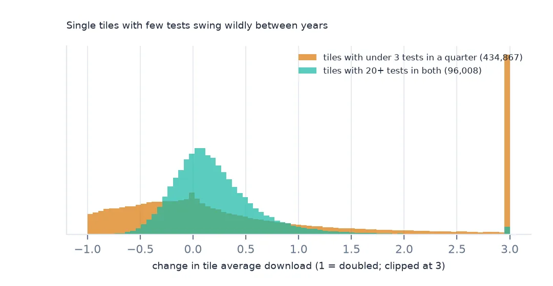
spread of change (IQR): tiles with under 3 tests 1.53; tiles with 20+ in both 0.46

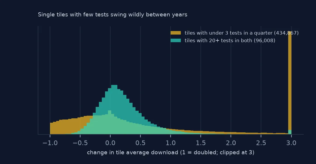
Single tiles are noisy. The middle half of changes spans 1.53 in tiles with fewer than 3 tests, against 0.46 in tiles with 20 or more tests in both quarters.

Overlapping histograms of the change in single-tile average download between years: tiles with few tests spread from minus 100% to over tripled, tiles with 20 or more tests in both years cluster near zero. — Single tiles with few tests swing wildly between years; well-tested tiles barely move.

3. By county

w = lambda d, col: wmedian(d[col], d.tests)
ca = fixed25.groupby("GEOID").apply(lambda d: pd.Series({"t": d.tests.sum(), "m": w(d, "avg_d_kbps") / 1000}), include_groups=False)
cb = fixed.groupby("GEOID").apply(lambda d: pd.Series({"t": d.tests.sum(), "m": w(d, "avg_d_kbps") / 1000}), include_groups=False)
cc = ca.join(cb, lsuffix="_25", rsuffix="_26").dropna()
cc = cc[(cc.t_25 >= 100) & (cc.t_26 >= 100)]
cc["change"] = cc.m_26 / cc.m_25 - 1
print(f"counties compared: {len(cc):,}; median change {cc.change.median():+.1%}; faster {(cc.change > 0).mean():.1%}")

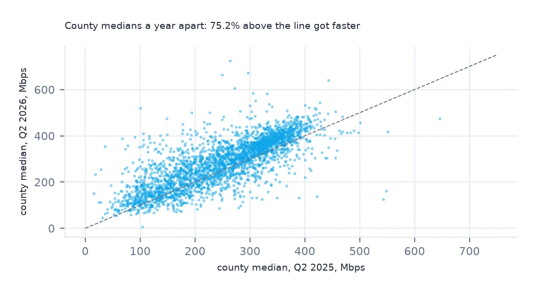
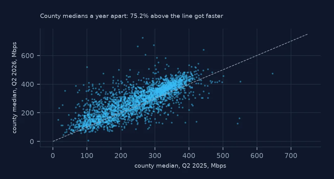
counties compared: 2,862; median change +12.6%; faster 75.2%

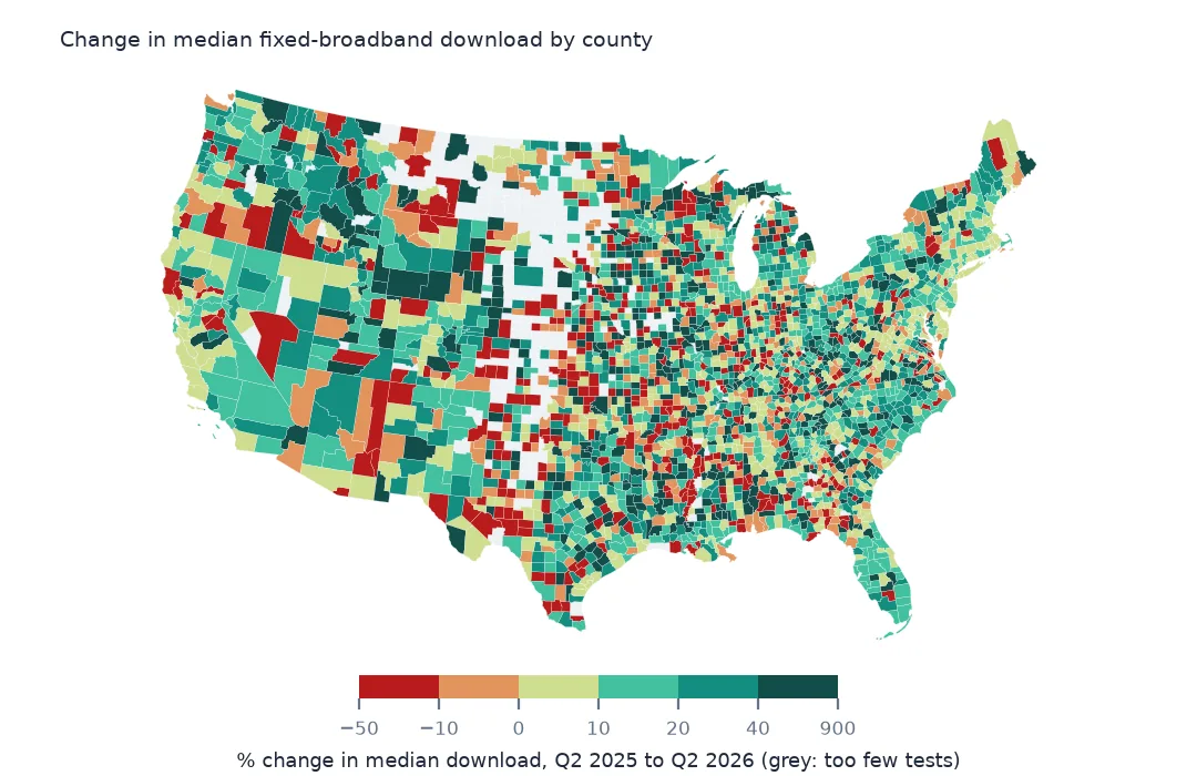
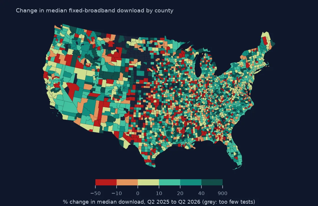
Among 2,862 counties with enough tests in both quarters, the median change is +12.6% and 75.2% got faster. County medians are steadier than tiles and still local enough to map.

Biggest rises and upload

The data used on this page

Ookla's Speedtest open data performance tiles for fixed broadband in April–June 2025 and April–June 2026, read from Amazon S3, and Census Bureau 2023 county boundaries.

from pathlib import Path

import duckdb
import geopandas as gpd
import numpy as np
import pandas as pd
import requests

Path("data").mkdir(exist_ok=True)
# Ookla Speedtest open data (AWS Open Data, keyless): one Parquet file per quarter and network type, zoom-16 web
# Mercator tiles with average speeds, latency, tests and devices. Published quarterly under fixed names.
BASE = "https://ookla-open-data.s3.amazonaws.com/parquet/performance"


def tiles(kind, year, q):
    """One quarter's tiles inside a box around the contiguous US, cached locally as Parquet."""
    path = f"data/ookla-{kind}-{year}q{q}-conus.parquet"
    if not Path(path).exists():
        url = f"{BASE}/type={kind}/year={year}/quarter={q}/{year}-{(q - 1) * 3 + 1:02d}-01_performance_{kind}_tiles.parquet"
        con = duckdb.connect()
        con.sql("INSTALL httpfs; LOAD httpfs;")
        con.sql(f"""COPY (SELECT quadkey, tile_x, tile_y, avg_d_kbps, avg_u_kbps, avg_lat_ms, avg_lat_down_ms, avg_lat_up_ms, tests, devices
                         FROM read_parquet('{url}') WHERE tile_x BETWEEN -125 AND -66 AND tile_y BETWEEN 24 AND 50
                         ORDER BY quadkey) TO '{path}' (FORMAT parquet)""")
    return pd.read_parquet(path)


for name in ["cb_2023_us_county_20m.zip"]:
    if not Path(f"data/{name}").exists():
        Path(f"data/{name}").write_bytes(requests.get(f"https://www2.census.gov/geo/tiger/GENZ2023/shp/{name}", timeout=300).content)
counties = gpd.read_file("data/cb_2023_us_county_20m.zip")
counties = counties[~counties.STUSPS.isin(["AK", "HI", "PR"])].to_crs(4326)


def in_counties(df):
    """Attach the county each tile's centre falls in; tiles outside the lower 48 (Canada, Mexico, sea) drop out."""
    pts = gpd.GeoDataFrame(df, geometry=gpd.points_from_xy(df.tile_x, df.tile_y), crs=4326)
    j = gpd.sjoin(pts, counties[["GEOID", "STUSPS", "NAME", "geometry"]], predicate="within")
    return pd.DataFrame(j.drop(columns=["geometry", "index_right"]))


def wmedian(values, weights):
    """Median of tile averages, each tile counted once per test."""
    o = np.argsort(values.to_numpy())
    v, w = values.to_numpy()[o], weights.to_numpy()[o]
    c = np.cumsum(w)
    return v[np.searchsorted(c, c[-1] / 2)]


fixed = in_counties(tiles("fixed", 2026, 2))
fixed25 = in_counties(tiles("fixed", 2025, 2))
print(f"Ookla fixed broadband, April-June 2026: {len(fixed):,} tiles in the lower 48, {fixed.tests.sum():,} tests")

Ookla fixed broadband, April-June 2026: 1,548,841 tiles in the lower 48, 15,134,971 tests

Example 1: the biggest rises

cc = cc.join(counties.set_index("GEOID")[["NAME", "STUSPS"]])
print(cc.sort_values("change").tail(4)[["NAME", "STUSPS", "m_25", "m_26"]].round(0).to_dict("records"))

[{'NAME': 'Washington', 'STUSPS': 'KS', 'm_25': 28.0, 'm_26': 256.0}, {'NAME': 'Humphreys', 'STUSPS': 'MS', 'm_25': 16.0, 'm_26': 151.0}, {'NAME': 'Morgan', 'STUSPS': 'OH', 'm_25': 36.0, 'm_26': 354.0}, {'NAME': 'Pawnee', 'STUSPS': 'OK', 'm_25': 18.0, 'm_26': 233.0}]

The biggest rises are from very low starting points: Washington County, Kansas went from 28 to 256 Mbps, and Humphreys County, Mississippi, Morgan County, Ohio and Pawnee County, Oklahoma rose similarly. Jumps like these point to a new network, typically fibre, reaching enough testers.

Scatter plot of county median download in Q2 2025 against Q2 2026 with an equality line; most points lie above it. — County medians a year apart: 75.2% of counties got faster.

Example 2: upload

print(f"upload: {wmedian(fixed25.avg_u_kbps, fixed25.tests) / 1000:.1f} -> {wmedian(fixed.avg_u_kbps, fixed.tests) / 1000:.1f} Mbps")

upload: 129.4 -> 150.1 Mbps

Upload rose faster than download, from 129.4 to 150.1 Mbps, as fibre, which is symmetrical, replaces cable and DSL.

Why speeds rise

Measured speeds rise when networks are upgraded (fibre replacing copper, cable plans raising tiers), when people buy faster plans, and when devices and Wi-Fi improve. Speedtest data cannot separate these. A county's median can also jump because a few dozen households on a new fibre network started testing. Year-on-year comparisons are strongest for large areas and for tiles with many tests in both periods.

Comparison pitfalls

Same quarter of the year avoids seasonal differences in who tests.
Matched tiles remove changes in where people tested, but drop new areas.
Weight changes by tests, not one vote per tile.
Big percentage jumps usually come from low starting points in small counties.

Internal links

How to map broadband speed by county — the county map
Average internet speed comes out wrong — weighting by tests
Empty Speedtest tiles — what absence means

FAQ

Did US internet speeds increase in 2026?

Yes: the tests-weighted median fixed-broadband download in the lower 48 rose from 341.0 Mbps in April–June 2025 to 381.2 Mbps in April–June 2026, 11.8%.

How do I compare Ookla speeds between quarters?

Read both quarters, compare tests-weighted medians, and for local change use tiles present in both or counties with enough tests in both.