How to Measure the Urban-Rural Broadband Speed Gap

Problem statement

Rural America's internet is slower than its cities', and billions in federal grants aim to close the gap. Ookla's open tiles let you measure it directly: group counties by population density and compare the speeds measured there. This page splits the lower 48's counties into five density classes, compares median download and upload, the share of tests below the FCC's 100/20 Mbps benchmark, and latency, and finds the states with the widest gap, using April–June 2026 data.

Quick answer

Compute each county's population density from Census estimates and land area, cut it into classes, attach the class to every tile, and compute tests-weighted medians and benchmark shares per class. Report upload as well as download: rural upload lags most.

area = counties.set_index("GEOID").to_crs(5070).area / 1e6
c = pd.DataFrame({"pop": pop, "km2": area}).dropna()
c["density"] = c["pop"] / c.km2
c["class"] = pd.cut(c.density, [0, 10, 50, 250, 1000, 1e6], labels=["under 10", "10-50", "50-250", "250-1,000", "1,000+"])
f = fixed.merge(c[["class"]], left_on="GEOID", right_index=True)
g = f.groupby("class", observed=True).apply(lambda d: pd.Series({"counties": d.GEOID.nunique(), "tests": d.tests.sum(), "mbps": wmedian(d.avg_d_kbps, d.tests) / 1000}), include_groups=False)
print(g.round(1).to_string())

           counties      tests   mbps
class                                
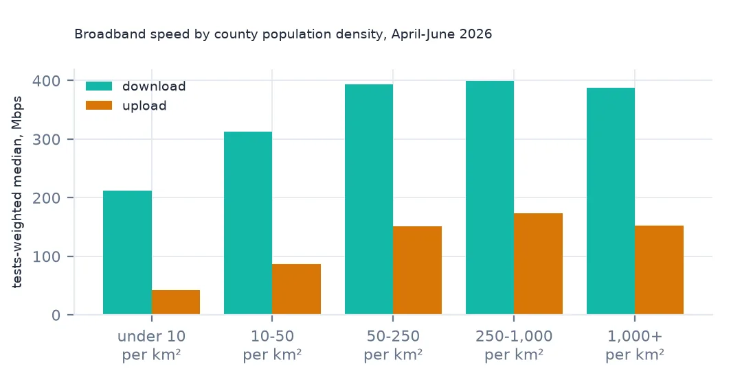
under 10     1092.0   639339.0  212.5
10-50        1276.0  2586429.0  313.2
50-250        529.0  4985735.0  393.0
250-1,000     166.0  5316129.0  399.5
1,000+         45.0  1607339.0  387.5

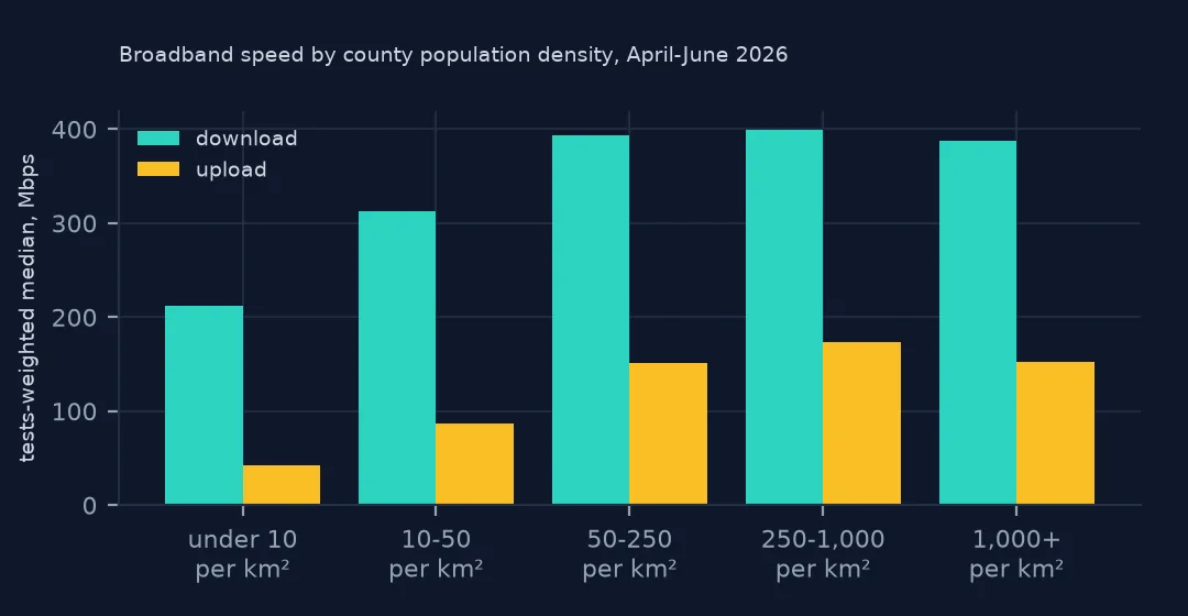
Median download rises with density from 212.5 Mbps in counties with under 10 people per km² to 393–400 Mbps in counties of 50–1,000. The densest counties are slightly slower (387.5 Mbps) than suburban ones, where newer fibre and cable networks are concentrated.

Density classes, benchmarks and upload

1. Population density classes

print(c["class"].value_counts().sort_index().to_dict())
print(f"people in counties under 50 per km2: {c[c.density < 50]['pop'].sum() / c['pop'].sum():.1%}")

{'under 10': 1093, '10-50': 1276, '50-250': 529, '250-1,000': 166, '1,000+': 45}
people in counties under 50 per km2: 20.7%

1,093 counties have under 10 people per km² and 45 over 1,000. Counties under 50 per km² hold 20.7% of the population, so the rural gap concerns about a fifth of Americans.

2. Share of tests below the 100/20 benchmark

f["below"] = (f.avg_d_kbps < 100_000) | (f.avg_u_kbps < 20_000)
print("share of tests below 100/20 Mbps:", f.groupby("class", observed=True).apply(lambda d: (d.below * d.tests).sum() / d.tests.sum(), include_groups=False).round(3).to_dict())

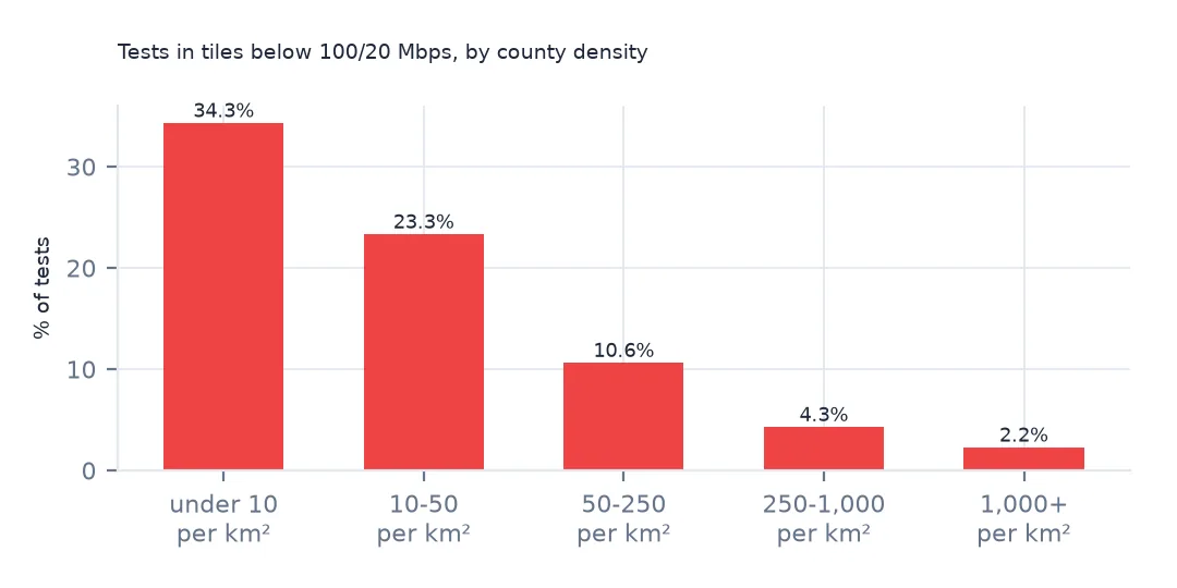
share of tests below 100/20 Mbps: {'under 10': 0.343, '10-50': 0.233, '50-250': 0.106, '250-1,000': 0.043, '1,000+': 0.022}

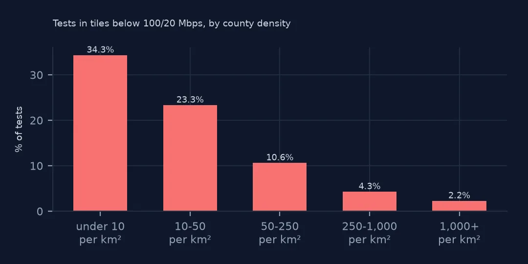
The share of tests in tiles below the FCC's 100/20 benchmark falls from 34.3% in the sparsest counties to 2.2% in the densest. A third of rural tests come from places without what the FCC now counts as broadband.

3. Within counties, by tile

f["tile_tests"] = f.tests
dense = f[f["class"] == "1,000+"]; sparse = f[f["class"] == "under 10"]
print(f"upload, dense counties {wmedian(dense.avg_u_kbps, dense.tests) / 1000:.0f} Mbps against sparse {wmedian(sparse.avg_u_kbps, sparse.tests) / 1000:.0f} Mbps")

upload, dense counties 152 Mbps against sparse 42 Mbps

Upload shows the gap most: 152 Mbps in the densest counties against 42 Mbps in the sparsest. Rural DSL, fixed wireless and satellite upload slowly.

States and latency

The data used on this page

Ookla's Speedtest open data performance tiles for fixed broadband (April–June 2026), read from Amazon S3, and Census Bureau 2023 county boundaries, and the Census Bureau's 2024 county population estimates.

from pathlib import Path

import duckdb
import geopandas as gpd
import numpy as np
import pandas as pd
import requests

Path("data").mkdir(exist_ok=True)
# Ookla Speedtest open data (AWS Open Data, keyless): one Parquet file per quarter and network type, zoom-16 web
# Mercator tiles with average speeds, latency, tests and devices. Published quarterly under fixed names.
BASE = "https://ookla-open-data.s3.amazonaws.com/parquet/performance"


def tiles(kind, year, q):
    """One quarter's tiles inside a box around the contiguous US, cached locally as Parquet."""
    path = f"data/ookla-{kind}-{year}q{q}-conus.parquet"
    if not Path(path).exists():
        url = f"{BASE}/type={kind}/year={year}/quarter={q}/{year}-{(q - 1) * 3 + 1:02d}-01_performance_{kind}_tiles.parquet"
        con = duckdb.connect()
        con.sql("INSTALL httpfs; LOAD httpfs;")
        con.sql(f"""COPY (SELECT quadkey, tile_x, tile_y, avg_d_kbps, avg_u_kbps, avg_lat_ms, avg_lat_down_ms, avg_lat_up_ms, tests, devices
                         FROM read_parquet('{url}') WHERE tile_x BETWEEN -125 AND -66 AND tile_y BETWEEN 24 AND 50
                         ORDER BY quadkey) TO '{path}' (FORMAT parquet)""")
    return pd.read_parquet(path)


for name in ["cb_2023_us_county_20m.zip"]:
    if not Path(f"data/{name}").exists():
        Path(f"data/{name}").write_bytes(requests.get(f"https://www2.census.gov/geo/tiger/GENZ2023/shp/{name}", timeout=300).content)
counties = gpd.read_file("data/cb_2023_us_county_20m.zip")
counties = counties[~counties.STUSPS.isin(["AK", "HI", "PR"])].to_crs(4326)


def in_counties(df):
    """Attach the county each tile's centre falls in; tiles outside the lower 48 (Canada, Mexico, sea) drop out."""
    pts = gpd.GeoDataFrame(df, geometry=gpd.points_from_xy(df.tile_x, df.tile_y), crs=4326)
    j = gpd.sjoin(pts, counties[["GEOID", "STUSPS", "NAME", "geometry"]], predicate="within")
    return pd.DataFrame(j.drop(columns=["geometry", "index_right"]))


def wmedian(values, weights):
    """Median of tile averages, each tile counted once per test."""
    o = np.argsort(values.to_numpy())
    v, w = values.to_numpy()[o], weights.to_numpy()[o]
    c = np.cumsum(w)
    return v[np.searchsorted(c, c[-1] / 2)]


fixed = in_counties(tiles("fixed", 2026, 2))
pop = pd.read_csv("https://www2.census.gov/programs-surveys/popest/datasets/2020-2024/counties/totals/co-est2024-alldata.csv",
                  encoding="latin-1", dtype={"STATE": str, "COUNTY": str}, usecols=["STATE", "COUNTY", "SUMLEV", "POPESTIMATE2024"])
pop = pop[pop.SUMLEV == 50].assign(GEOID=lambda d: d.STATE + d.COUNTY).set_index("GEOID").POPESTIMATE2024
print(f"Ookla fixed broadband, April-June 2026: {len(fixed):,} tiles in the lower 48, {fixed.tests.sum():,} tests")

Ookla fixed broadband, April-June 2026: 1,548,841 tiles in the lower 48, 15,134,971 tests

Example 1: states with the widest gap

f["rural"] = f["class"].isin(["under 10", "10-50"])
s = f.groupby(["STUSPS", "rural"]).apply(lambda d: wmedian(d.avg_d_kbps, d.tests) / 1000, include_groups=False).unstack()
s = s.dropna(); s["gap"] = s[False] - s[True]
print(s.sort_values("gap").tail(4).round(0).to_dict("index"))

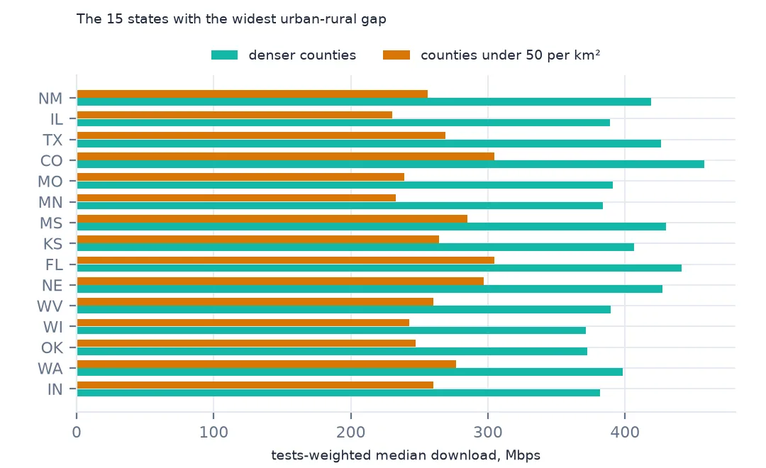
{'CO': {False: 458.0, True: 305.0, 'gap': 153.0}, 'TX': {False: 426.0, True: 269.0, 'gap': 157.0}, 'IL': {False: 389.0, True: 230.0, 'gap': 159.0}, 'NM': {False: 419.0, True: 256.0, 'gap': 163.0}}

Among states with both kinds of county, the gap between non-rural and rural medians is widest in New Mexico (163 Mbps), Illinois, Texas and Colorado.

Example 2: latency

print(f.groupby("class", observed=True).apply(lambda d: wmedian(d.avg_lat_ms, d.tests), include_groups=False).to_dict())

{'under 10': 19, '10-50': 15, '50-250': 13, '250-1,000': 11, '1,000+': 10}

Latency follows density too, from 19 ms in the sparsest counties to 10 ms in the densest. Distance to the nearest internet exchange adds milliseconds, and satellite links add more.

Why rural internet is slower

Building wired networks costs roughly the same per kilometre of road whether it passes ten homes or a thousand, so sparse areas were left with old telephone copper, fixed wireless or satellite. Cable and fibre arrived in towns first. Recent programmes (USDA ReConnect, the FCC's Rural Digital Opportunity Fund and BEAD) fund rural fibre, which is why some of the fastest counties in the data are rural. The gap is shrinking where networks are built and remains wide where they are not.

Measuring the gap

• Density by county is coarse: rural tracts inside metro counties are averaged with the city.
• Use upload and the 100/20 benchmark, not just median download.
• Rural tiles have fewer tests, so their medians are noisier.
• Satellite (including low-orbit services) counts as fixed broadband here.

Internal links

• How to map broadband speed by county — the county map
• Speedtest data explained — who runs tests
• How to compare mobile and fixed speeds — the two networks

FAQ

How much slower is rural internet in the US?

In April–June 2026, counties with under 10 people per km² had a tests-weighted median download of 212.5 Mbps, against 393–400 Mbps in counties of 50–1,000 per km².

What share of rural speed tests miss the 100/20 Mbps benchmark?

34.3% of tests in counties under 10 people per km², against 2.2% in counties over 1,000 per km².