How to Read Ookla Speedtest Open Data Tiles in Python

Problem statement

Ookla publishes the results of its Speedtest app every quarter as open data: the whole world divided into small map tiles, each with the average download and upload speed, latency, and the number of tests and devices behind it. It is the most detailed public picture of real internet speeds, free on Amazon S3 with no key. The files are large (hundreds of megabytes a quarter), speeds are in kilobits, and each row is a tile average, not a test. This page reads the April–June 2026 fixed-broadband tiles for the contiguous US with DuckDB, explains every field, and builds a tile layer.

Quick answer

Query the quarter's Parquet file on S3 with DuckDB (read_parquet with the httpfs extension), filtering on tile_x and tile_y so only the region's row groups are read. Divide avg_d_kbps and avg_u_kbps by 1,000 for Mbps, and weight by tests when combining tiles.

print(fixed[["quadkey", "tile_x", "tile_y", "avg_d_kbps", "avg_u_kbps", "avg_lat_ms", "tests", "devices"]].head(3).to_string(index=False))
print(f"tests-weighted median download {wmedian(fixed.avg_d_kbps, fixed.tests) / 1000:.1f} Mbps, upload {wmedian(fixed.avg_u_kbps, fixed.tests) / 1000:.1f} Mbps")

         quadkey    tile_x  tile_y  avg_d_kbps  avg_u_kbps  avg_lat_ms  tests  devices
0212122232312121 -122.7530 49.0000      481959      115700          11      4        2
0212122232312123 -122.7530 48.9964       35935        8503          18      6        6
0212122232312130 -122.7475 49.0000      330967      197841          13      5        5
tests-weighted median download 381.2 Mbps, upload 150.1 Mbps

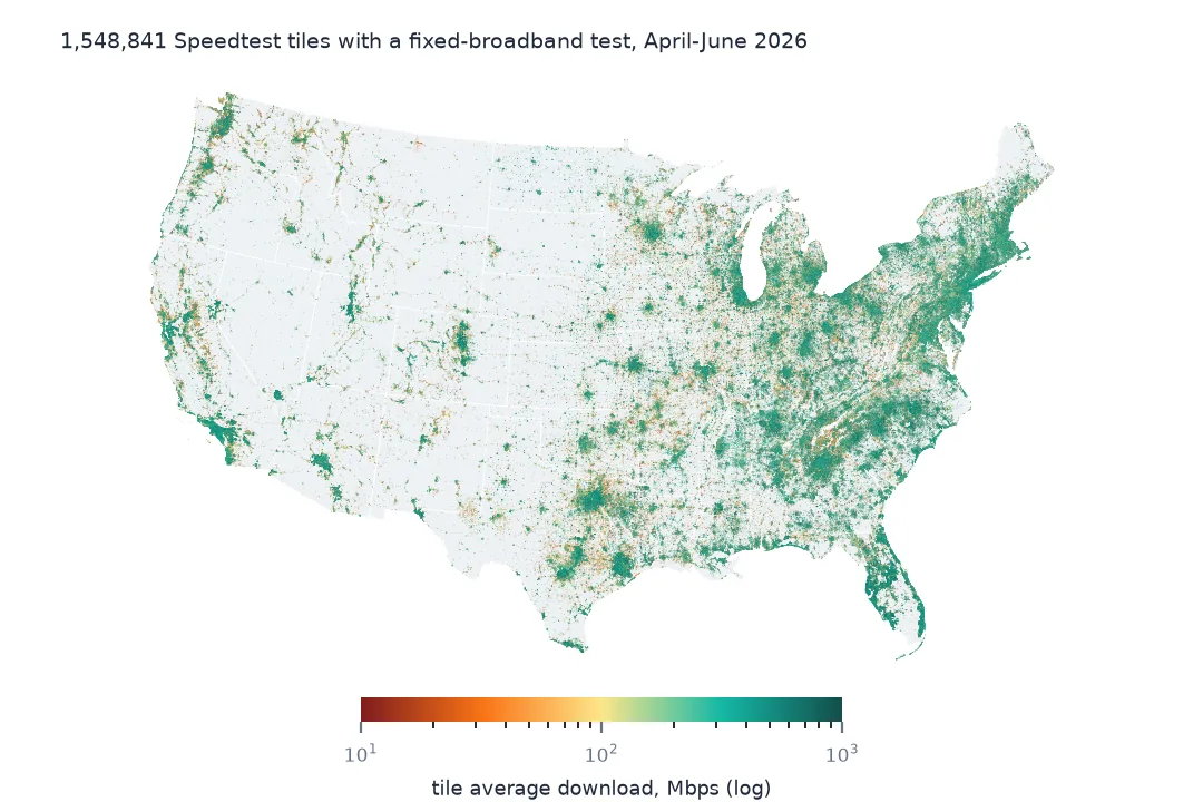
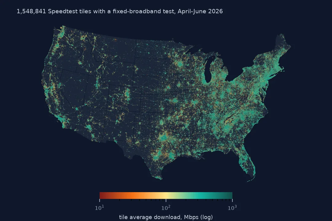
Each row is one tile: its quadkey, centre, average download and upload in kilobits per second, idle latency, and the tests and devices behind it. Counting each test once, the median fixed-broadband download in the lower 48 is 381.2 Mbps and upload 150.1 Mbps.

Tiles, units, tests and polygons

1. One row per zoom-16 tile

print(f"quadkey length: {fixed.quadkey.str.len().unique().tolist()}; tile size at 40N: {40075 / 2 ** 16 * np.cos(np.radians(40)) * 1000:.0f} m")
print(f"tiles: {len(fixed):,}; counties with at least one: {fixed.GEOID.nunique():,} of {len(counties):,}")

quadkey length: [16]; tile size at 40N: 468 m
tiles: 1,548,841; counties with at least one: 3,108 of 3,109

Quadkeys are 16 digits, so tiles are zoom 16, about 468 m across at 40°N and smaller further north. The lower 48 have 1,548,841 tiles with at least one fixed-broadband test this quarter, in 3,108 of 3,109 counties.

2. Speeds are kilobits per second

print(fixed[["avg_d_kbps", "avg_u_kbps"]].describe(percentiles=[0.5]).loc[["min", "50%", "max"]].to_string())

     avg_d_kbps  avg_u_kbps
min         1.0         1.0
50%    310440.0     74286.0
max   8081744.0   7668815.0

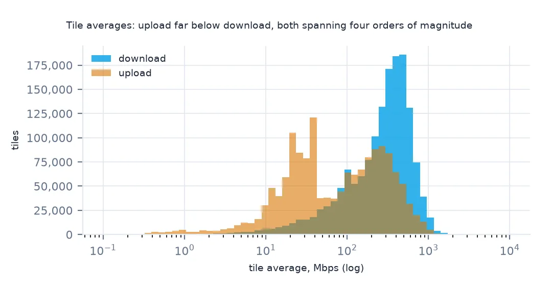
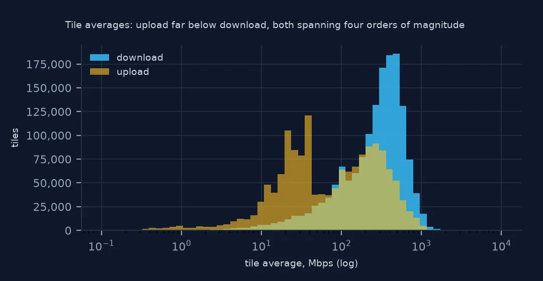
Tile averages range from 1 kbps to 8,081,744 kbps (8 Gbps). The median tile averages 310,440 kbps down and 74,286 kbps up.

3. Tests and devices

print(f"tests per tile: median {fixed.tests.median():.0f}, max {fixed.tests.max():,}; devices per tile: median {fixed.devices.median():.0f}")
print(f"tiles with a single test: {(fixed.tests == 1).mean():.1%}")

tests per tile: median 3, max 61,249; devices per tile: median 2
tiles with a single test: 28.4%

The median tile has 3 tests from 2 devices, and 28.4% have a single test. The busiest has 61,249. A tile average from one test is one person's measurement on one evening.

4. Tile polygons

x0, y0 = fixed.iloc[0][["tile_x", "tile_y"]]
con = duckdb.connect(); con.sql("INSTALL httpfs; LOAD httpfs;")
url = f"{BASE}/type=fixed/year=2026/quarter=2/2026-04-01_performance_fixed_tiles.parquet"
row = con.sql(f"SELECT quadkey, tile FROM read_parquet('{url}') WHERE quadkey = '{fixed.iloc[0].quadkey}'").fetchone()
print(row[0], row[1][:120])

0212122232312121 POLYGON((-122.755737304688 49.0018439179785, -122.750244140625 49.0018439179785, -122.750244140625 48.9982400811387, -12

The tile column stores each tile as a WKT polygon, a square in web Mercator that is slightly taller than wide in degrees. Reading it for a single quadkey takes a moment because DuckDB fetches only the matching row group.

States and a tile layer

The data used on this page

Ookla's Speedtest open data performance tiles for fixed broadband (April–June 2026), read from Amazon S3, and Census Bureau 2023 county boundaries.

from pathlib import Path

import duckdb
import geopandas as gpd
import numpy as np
import pandas as pd
import requests

Path("data").mkdir(exist_ok=True)
# Ookla Speedtest open data (AWS Open Data, keyless): one Parquet file per quarter and network type, zoom-16 web
# Mercator tiles with average speeds, latency, tests and devices. Published quarterly under fixed names.
BASE = "https://ookla-open-data.s3.amazonaws.com/parquet/performance"


def tiles(kind, year, q):
    """One quarter's tiles inside a box around the contiguous US, cached locally as Parquet."""
    path = f"data/ookla-{kind}-{year}q{q}-conus.parquet"
    if not Path(path).exists():
        url = f"{BASE}/type={kind}/year={year}/quarter={q}/{year}-{(q - 1) * 3 + 1:02d}-01_performance_{kind}_tiles.parquet"
        con = duckdb.connect()
        con.sql("INSTALL httpfs; LOAD httpfs;")
        con.sql(f"""COPY (SELECT quadkey, tile_x, tile_y, avg_d_kbps, avg_u_kbps, avg_lat_ms, avg_lat_down_ms, avg_lat_up_ms, tests, devices
                         FROM read_parquet('{url}') WHERE tile_x BETWEEN -125 AND -66 AND tile_y BETWEEN 24 AND 50
                         ORDER BY quadkey) TO '{path}' (FORMAT parquet)""")
    return pd.read_parquet(path)


for name in ["cb_2023_us_county_20m.zip"]:
    if not Path(f"data/{name}").exists():
        Path(f"data/{name}").write_bytes(requests.get(f"https://www2.census.gov/geo/tiger/GENZ2023/shp/{name}", timeout=300).content)
counties = gpd.read_file("data/cb_2023_us_county_20m.zip")
counties = counties[~counties.STUSPS.isin(["AK", "HI", "PR"])].to_crs(4326)


def in_counties(df):
    """Attach the county each tile's centre falls in; tiles outside the lower 48 (Canada, Mexico, sea) drop out."""
    pts = gpd.GeoDataFrame(df, geometry=gpd.points_from_xy(df.tile_x, df.tile_y), crs=4326)
    j = gpd.sjoin(pts, counties[["GEOID", "STUSPS", "NAME", "geometry"]], predicate="within")
    return pd.DataFrame(j.drop(columns=["geometry", "index_right"]))


def wmedian(values, weights):
    """Median of tile averages, each tile counted once per test."""
    o = np.argsort(values.to_numpy())
    v, w = values.to_numpy()[o], weights.to_numpy()[o]
    c = np.cumsum(w)
    return v[np.searchsorted(c, c[-1] / 2)]


fixed = in_counties(tiles("fixed", 2026, 2))
print(f"Ookla fixed broadband, April-June 2026: {len(fixed):,} tiles in the lower 48, {fixed.tests.sum():,} tests")

Ookla fixed broadband, April-June 2026: 1,548,841 tiles in the lower 48, 15,134,971 tests

Example 1: by state

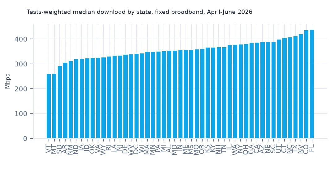
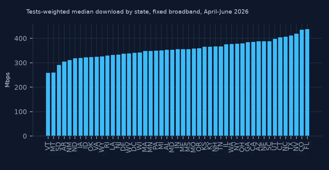
st = fixed.groupby("STUSPS").apply(lambda g: pd.Series({"tiles": len(g), "tests": g.tests.sum(), "median_mbps": wmedian(g.avg_d_kbps, g.tests) / 1000}), include_groups=False)
print(st.sort_values("median_mbps").iloc[[0, 1, 2, -3, -2, -1]].round(1).to_string())

          tiles      tests  median_mbps
STUSPS                                 
VT       6706.0    30132.0        258.4
MT      10094.0    50609.0        260.2
SD       4967.0    25667.0        290.5
NV       9838.0   192605.0        419.4
CO      30094.0   354756.0        434.7
FL      84499.0  1271951.0        437.6

By state, Vermont (258.4 Mbps), Montana and South Dakota have the slowest tests-weighted medians, and Nevada, Colorado and Florida (437.6 Mbps) the fastest, among the six shown. Florida also has by far the most tests (1,271,951).

Example 2: a tile layer for one city

from shapely.geometry import box
d = 360 / 2 ** 16
den = fixed[(fixed.STUSPS == "CO") & fixed.NAME.isin(["Denver"])]
g = gpd.GeoDataFrame(den[["quadkey", "avg_d_kbps", "tests"]], crs=4326,
                     geometry=[box(x - d / 2, y - d / 2 * np.cos(np.radians(y)), x + d / 2, y + d / 2 * np.cos(np.radians(y))) for x, y in zip(den.tile_x, den.tile_y)])
g.to_file("denver_tiles.gpkg", driver="GPKG")
print(f"{len(g):,} Denver tiles written; {g.tests.sum():,} tests")

1,348 Denver tiles written; 37,532 tests

1,348 Denver tiles with 37,532 tests make a small GeoPackage of squares. The squares here are built from the centres, which is quicker than parsing the WKT column and accurate enough for maps.

Where the tiles come from

Every Speedtest run records the device's location, and Ookla aggregates the quarter's tests into zoom-16 web Mercator tiles, identified by a 16-digit quadkey. For each tile it publishes the mean download and upload speed, mean latency (idle and under load), and how many tests and distinct devices contributed. Locations are approximate, tiles with no tests are simply absent, and speeds are averages of whatever tests people chose to run, which is why the averages need care.

Reading the files efficiently

• Filter on tile_x/tile_y, the tile centre, to read only part of a file over HTTP.
• The tile column holds each polygon as WKT; skip it unless you need the exact squares, as it is the largest column.
• Cache the subset locally (this page writes a Parquet per quarter) instead of querying S3 every run.
• File names are fixed per quarter and the published quarters do not change, so live reads reproduce.

Internal links

• Speedtest data explained — who runs tests
• Internet speeds a thousand times too high — kilobits
• Average internet speed comes out wrong — weighting by tests
• How to use quadkeys as a tile index — the tile scheme

FAQ

How do I download Ookla Speedtest open data?

From the public S3 bucket ookla-open-data, one Parquet file per quarter and network type, for example parquet/performance/type=fixed/year=2026/quarter=2/2026-04-01_performance_fixed_tiles.parquet. No account or key is needed.

What is the median broadband speed in the US?

In Ookla's fixed-broadband tiles for April–June 2026, the tests-weighted median download in the lower 48 is 381.2 Mbps and upload 150.1 Mbps.