Speedtest Data Explained: Who Runs Tests and What the Averages Mean

Problem statement

Speedtest data is crowdsourced: a tile's average is whatever tests people chose to run there. People test when something seems wrong, when they have just upgraded, when they are curious, or when an app runs a test for them. Some places produce dozens of tests per thousand residents and others few, and a single device can run many tests in one tile. This page measures who tests, how concentrated the tests are, and what that means for any average built from the tiles, using the April–June 2026 fixed-broadband data for the lower 48.

Quick answer

Treat Speedtest averages as measurements of the tests people ran, not of every household. Weight by tests, report how many tests stand behind each figure, and avoid conclusions from places with few tests. Compare with other sources (the FCC's National Broadband Map, ACS subscription data) before claiming coverage or the lack of it.

c = fixed.groupby("GEOID").agg(tests=("tests", "sum"), tiles=("quadkey", "size"))
c = c.join(pop.rename("pop"), how="inner")
c["tests_per_1000"] = c.tests / c["pop"] * 1000
print(f"tests per 1,000 residents by county: median {c.tests_per_1000.median():.1f}, 10th percentile {c.tests_per_1000.quantile(0.1):.1f}, 90th {c.tests_per_1000.quantile(0.9):.1f}")

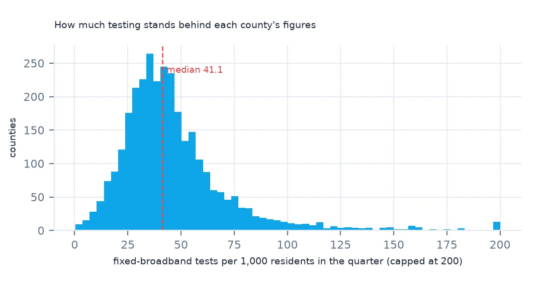
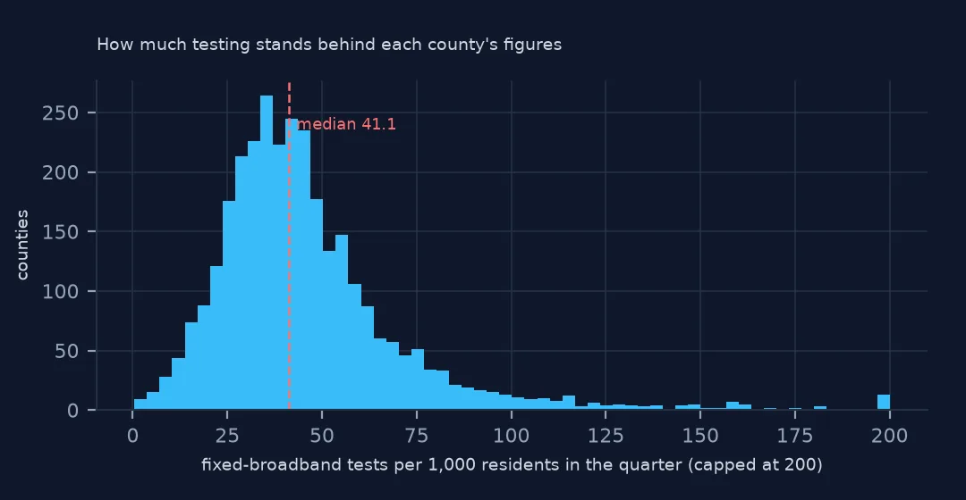
tests per 1,000 residents by county: median 41.1, 10th percentile 22.1, 90th 75.1

The median county produced 41.1 fixed-broadband tests per 1,000 residents in the quarter, but the spread is wide: 22.1 at the 10th percentile and 75.1 at the 90th. A county's average rests on very different amounts of evidence depending on where it is.

Tests per device, concentration and who tests

1. Tests per device

r = fixed.tests / fixed.devices
print(f"tests per device in a tile: median {r.median():.2f}, mean {r.mean():.2f}; tiles where one device ran 10+ tests: {(fixed.devices.eq(1) & fixed.tests.ge(10)).sum():,}")

tests per device in a tile: median 2.00, mean 3.06; tiles where one device ran 10+ tests: 31,850

The median tile has 2.00 tests per device and the mean 3.06. In 31,850 tiles a single device ran 10 or more tests: one household's troubleshooting session sets the whole tile's average.

2. Concentration of tests

s = fixed.tests.sort_values(ascending=False)
print(f"top 1% of tiles: {s.head(len(s) // 100).sum() / s.sum():.1%} of tests; tiles with one test: {(fixed.tests == 1).mean():.1%}")

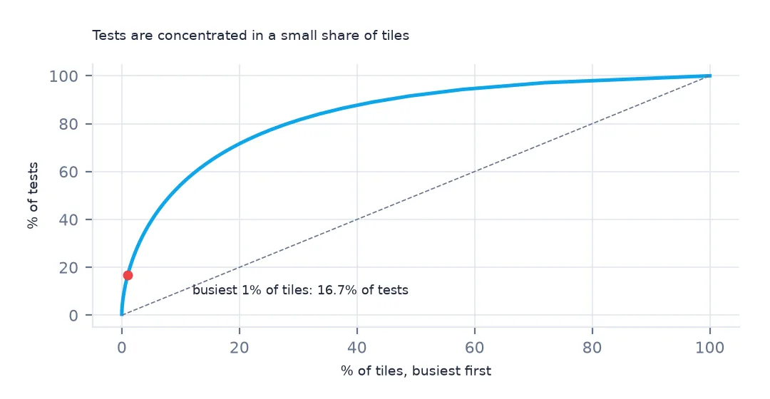
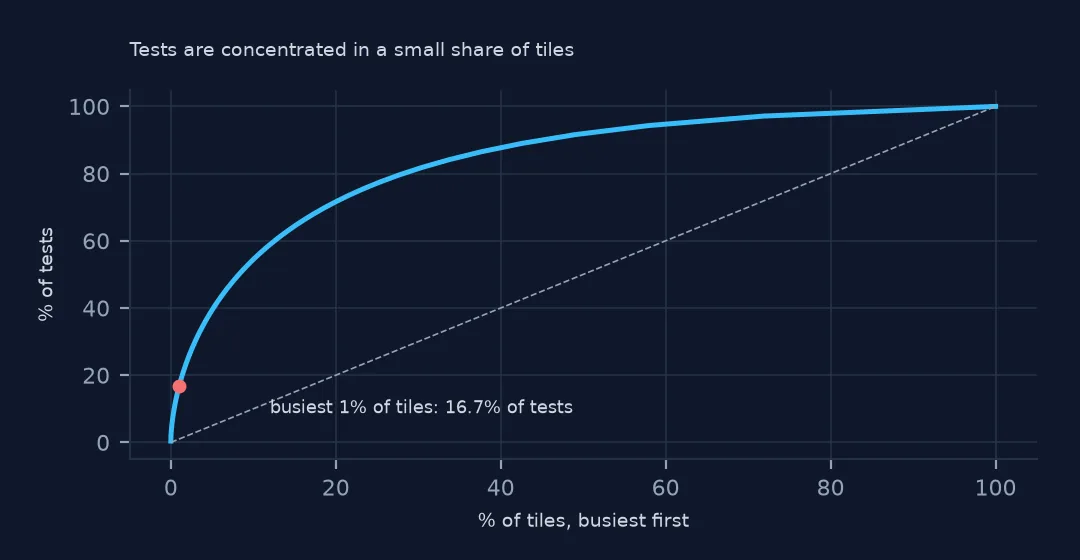
top 1% of tiles: 16.7% of tests; tiles with one test: 28.4%

The busiest 1% of tiles hold 16.7% of all tests, and 28.4% of tiles have just one. Unweighted tile statistics give the one-test tiles as much say as the busiest.

3. Who tests more

c["density"] = c["pop"] / (counties.set_index("GEOID").to_crs(5070).area / 1e6).reindex(c.index)
print(f"rank correlation of tests per resident with population density: {c.tests_per_1000.corr(c.density, method='spearman'):.2f}")
c["mbps"] = fixed.groupby("GEOID").apply(lambda g: wmedian(g.avg_d_kbps, g.tests), include_groups=False) / 1000
print(f"rank correlation of tests per resident with county median speed: {c.tests_per_1000.corr(c.mbps, method='spearman'):.2f}")

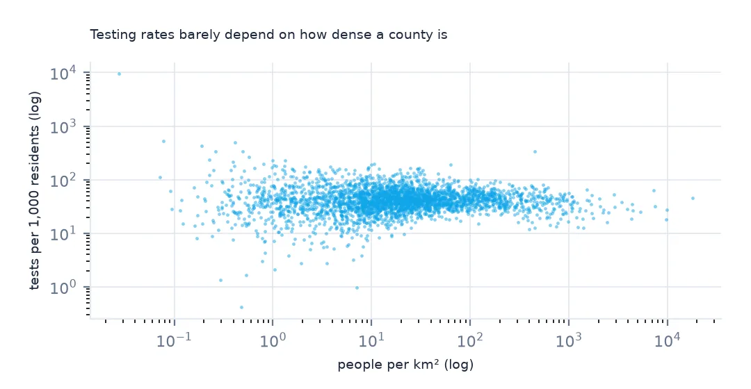
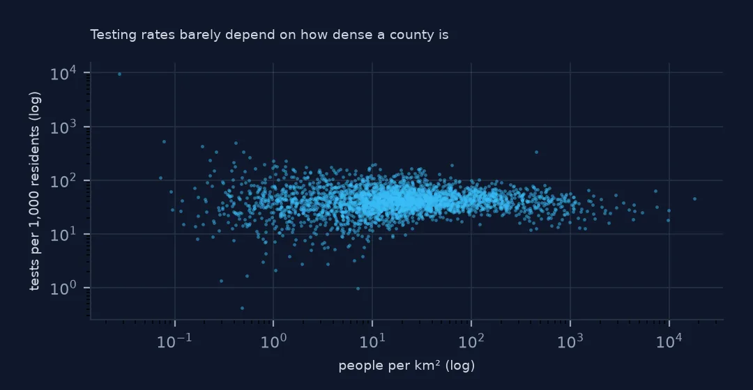
rank correlation of tests per resident with population density: 0.05
rank correlation of tests per resident with county median speed: 0.08

Testing is not much more common in dense counties (rank correlation 0.05 with population density) or in fast ones (0.08 with the county's median speed). The bias is less about place than about the reasons people test, which vary within every county.

Slow tiles and thin counties

The data used on this page

Ookla's Speedtest open data performance tiles for fixed broadband (April–June 2026), read from Amazon S3, and Census Bureau 2023 county boundaries, and the Census Bureau's 2024 county population estimates.

from pathlib import Path

import duckdb
import geopandas as gpd
import numpy as np
import pandas as pd
import requests

Path("data").mkdir(exist_ok=True)
# Ookla Speedtest open data (AWS Open Data, keyless): one Parquet file per quarter and network type, zoom-16 web
# Mercator tiles with average speeds, latency, tests and devices. Published quarterly under fixed names.
BASE = "https://ookla-open-data.s3.amazonaws.com/parquet/performance"


def tiles(kind, year, q):
    """One quarter's tiles inside a box around the contiguous US, cached locally as Parquet."""
    path = f"data/ookla-{kind}-{year}q{q}-conus.parquet"
    if not Path(path).exists():
        url = f"{BASE}/type={kind}/year={year}/quarter={q}/{year}-{(q - 1) * 3 + 1:02d}-01_performance_{kind}_tiles.parquet"
        con = duckdb.connect()
        con.sql("INSTALL httpfs; LOAD httpfs;")
        con.sql(f"""COPY (SELECT quadkey, tile_x, tile_y, avg_d_kbps, avg_u_kbps, avg_lat_ms, avg_lat_down_ms, avg_lat_up_ms, tests, devices
                         FROM read_parquet('{url}') WHERE tile_x BETWEEN -125 AND -66 AND tile_y BETWEEN 24 AND 50
                         ORDER BY quadkey) TO '{path}' (FORMAT parquet)""")
    return pd.read_parquet(path)


for name in ["cb_2023_us_county_20m.zip"]:
    if not Path(f"data/{name}").exists():
        Path(f"data/{name}").write_bytes(requests.get(f"https://www2.census.gov/geo/tiger/GENZ2023/shp/{name}", timeout=300).content)
counties = gpd.read_file("data/cb_2023_us_county_20m.zip")
counties = counties[~counties.STUSPS.isin(["AK", "HI", "PR"])].to_crs(4326)


def in_counties(df):
    """Attach the county each tile's centre falls in; tiles outside the lower 48 (Canada, Mexico, sea) drop out."""
    pts = gpd.GeoDataFrame(df, geometry=gpd.points_from_xy(df.tile_x, df.tile_y), crs=4326)
    j = gpd.sjoin(pts, counties[["GEOID", "STUSPS", "NAME", "geometry"]], predicate="within")
    return pd.DataFrame(j.drop(columns=["geometry", "index_right"]))


def wmedian(values, weights):
    """Median of tile averages, each tile counted once per test."""
    o = np.argsort(values.to_numpy())
    v, w = values.to_numpy()[o], weights.to_numpy()[o]
    c = np.cumsum(w)
    return v[np.searchsorted(c, c[-1] / 2)]


fixed = in_counties(tiles("fixed", 2026, 2))
pop = pd.read_csv("https://www2.census.gov/programs-surveys/popest/datasets/2020-2024/counties/totals/co-est2024-alldata.csv",
                  encoding="latin-1", dtype={"STATE": str, "COUNTY": str}, usecols=["STATE", "COUNTY", "SUMLEV", "POPESTIMATE2024"])
pop = pop[pop.SUMLEV == 50].assign(GEOID=lambda d: d.STATE + d.COUNTY).set_index("GEOID").POPESTIMATE2024
print(f"Ookla fixed broadband, April-June 2026: {len(fixed):,} tiles in the lower 48, {fixed.tests.sum():,} tests")

Ookla fixed broadband, April-June 2026: 1,548,841 tiles in the lower 48, 15,134,971 tests

Example 1: the slowest tests

slow = fixed[fixed.avg_d_kbps < 25_000]
print(f"tiles averaging under 25 Mbps: {len(slow) / len(fixed):.1%} of tiles, {slow.tests.sum() / fixed.tests.sum():.1%} of tests")

tiles averaging under 25 Mbps: 4.3% of tiles, 1.1% of tests

Tiles averaging under 25 Mbps are 4.3% of tiles but only 1.1% of tests: slow tiles tend to have few tests. Counting tiles overstates how common slow service is, and counting tests understates it if slow-line households test less.

Example 2: medians from few tests

small = c[c.tests < 100]
print(f"counties with fewer than 100 tests in the quarter: {len(small)}; their total population {small['pop'].sum():,}")

counties with fewer than 100 tests in the quarter: 201; their total population 665,209

201 counties had fewer than 100 tests in the quarter, home to 665,209 people. Their medians are the least reliable figures on any county map.

Why crowdsourced speeds are biased

Speed tests are run by self-selected users at self-selected moments. Users who suspect a problem test more, so slow connections can be over-represented; enthusiasts with new fibre test to show it off; and test results reflect the user's Wi-Fi and device as much as the line. Households that cannot afford broadband run no tests at all. Ookla's aggregation reduces some noise (it reports devices separately and drops obvious errors), but no tile average is a random sample of households. The data is excellent for comparing places with many tests and weak for small counties or for estimating who has access at all.

Using the tests honestly

• Show test counts beside every speed figure.
• Prefer medians weighted by tests over plain tile averages.
• Do not map absence as no service; it means no tests.
• Compare quarters carefully: test volumes change with app releases and outages.

Internal links

• How to read Ookla Speedtest tiles — the files and fields
• Average internet speed comes out wrong — weighting by tests
• Empty Speedtest tiles — what absence means

FAQ

Is Speedtest data representative?

Not of all households: it reflects who chose to run tests. In April–June 2026 the median county produced 41.1 tests per 1,000 residents, and 201 counties had fewer than 100 tests in the quarter.

How many Speedtest tests are behind Ookla's open data?

15,134,971 fixed-broadband tests in the lower 48 in April–June 2026, spread over 1,548,841 tiles.