How to Analyse New York's Street Tree Census in Python

Problem statement

In 2015 and 2016 New York City counted every tree on its streets: 683,788 records, each with a location, a species, a trunk diameter, a health rating and a checklist of problems, collected by city staff, census staff and volunteers. It is one of the largest open urban-tree datasets anywhere and a model for what a street tree inventory can hold.

It also has the habits of a big field survey. The coordinates come in two systems, one in US survey feet; dead trees and stumps share the file with living ones; a few fields are lists in a single string; and pandas reads the word "None", written thousands of times in it, as missing data. This page loads the census, builds a projected GeoDataFrame, and checks each of those before any analysis.

Quick answer

Keep living trees, build points from the State Plane coordinates (EPSG:2263, feet), reproject to the metric New York Long Island zone (EPSG:32118), and summarise:

import geopandas as gpd

alive = trees[trees.status == "Alive"]
gdf = gpd.GeoDataFrame(alive, geometry=gpd.points_from_xy(alive.x_sp, alive.y_sp), crs=2263).to_crs(32118)
print(gdf.crs.name, "| units:", gdf.crs.axis_info[0].unit_name)
print(alive.groupby("borough").agg(trees=("tree_id", "size"), species=("spc_common", "nunique"),
                                   median_dbh_in=("tree_dbh", "median")).to_string())

NAD83 / New York Long Island | units: metre
                trees  species  median_dbh_in
borough                                      
Bronx           80585      132            8.0
Brooklyn       169744      132           10.0
Manhattan       62427      128            8.0
Queens         237974      132           11.0
Staten Island  101443      131            9.0

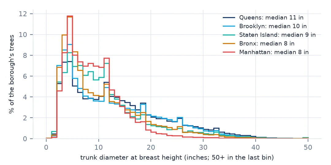
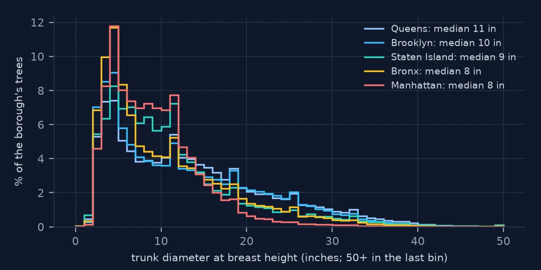
652,173 living street trees, from 62,427 in Manhattan to 237,974 in Queens, and 128 to 132 species in every borough. Queens' trees are the largest, with a median trunk diameter of 11 inches against 8 in the Bronx and Manhattan. Reprojecting to EPSG:32118 means every distance from here on is in metres.

Rows, coordinates, species and size

1. What a row is

print(trees.status.value_counts().to_string())
print(trees.groupby("status")[["spc_common", "health", "tree_dbh", "stump_diam"]].apply(lambda g: g.notna().mean()).round(2).to_string())
print(trees.tree_id.is_unique, "unique tree ids;", trees.block_id.nunique(), "block ids")

status
Alive    652173
Stump     17654
Dead      13961
        spc_common  health  tree_dbh  stump_diam
status                                          
Alive          1.0     1.0       1.0         1.0
Dead           0.0     0.0       1.0         1.0
Stump          0.0     0.0       1.0         1.0
True unique tree ids; 101390 block ids

Besides the living trees the census recorded 17,654 stumps and 13,961 dead trees. They have no species and no health, but they are planting sites — a stump is a place where a tree stood. Each record has a unique tree_id, and 101,390 block_ids group the trees by city block.

2. Two sets of coordinates, one in feet

from pyproj import Transformer

lon, lat = Transformer.from_crs(2263, 4326, always_xy=True).transform(trees.x_sp.values, trees.y_sp.values)
gap_m = np.hypot((lat - trees.latitude) * 111_320, (lon - trees.longitude) * 111_320 * np.cos(np.radians(40.7)))
print(f"State Plane x/y against latitude/longitude: median {np.median(gap_m):.2f} m, max {gap_m.max():.1f} m apart")
print(f"x_sp spans {trees.x_sp.min():,.0f} to {trees.x_sp.max():,.0f} — US survey feet, EPSG:2263")

State Plane x/y against latitude/longitude: median 0.00 m, max 0.0 m apart
x_sp spans 913,349 to 1,067,248 — US survey feet, EPSG:2263

The State Plane coordinates and the latitude and longitude agree exactly: they are the same point in two systems. The State Plane values are US survey feet — x_sp runs to over a million — so anything measured with them directly comes out in feet. Reprojecting to a metric CRS avoids that.

3. Species: common names and the missing ones

top = alive.spc_common.value_counts()
print(f"{alive.spc_common.nunique()} species; the top five:")
print((100 * top.head(5) / len(alive)).round(1).to_string())
print("alive trees without a species:", alive.spc_common.isna().sum())

132 species; the top five:
spc_common
London planetree    13.3
honeylocust          9.9
Callery pear         9.0
pin oak              8.2
Norway maple         5.2
alive trees without a species: 5

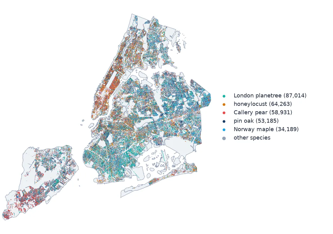
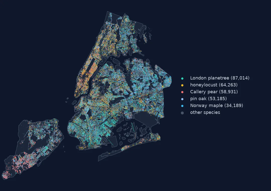
One species, the London planetree, is 13.3% of all living street trees, and five species make up almost half. Only 5 living trees have no species recorded.

4. Size, health and problems

print(alive.tree_dbh.describe(percentiles=[0.5, 0.9, 0.99]).round(1).to_string())
print(alive.health.value_counts(normalize=True).round(3).to_dict())
print(f"problems field filled for {alive.problems.notna().mean():.1%} of living trees; empty means none recorded")

count    652173.0
mean         11.7
std           8.6
min           0.0
50%          10.0
90%          24.0
99%          37.0
max         425.0
{'Good': 0.811, 'Fair': 0.148, 'Poor': 0.041}
problems field filled for 34.6% of living trees; empty means none recorded

Trunk diameters have a median of 10 inches and a 99th percentile of 37 — and a maximum of 425, a tree 35 feet across, which no street tree is (impossible diameters). 81.1% of living trees were rated Good. The problems field is filled for only 34.6% of trees: not because two-thirds were not inspected, but because the rest say "None", which pandas reads as missing (street tree censuses explained shows the word in the file).

Boroughs and recorders

The data used on this page

New York City Department of Parks and Recreation, TreesCount! 2015 Street Tree Census on NYC Open Data: one row for every street tree, stump and dead tree mapped by staff and volunteers in 2015–2016, with species, trunk diameter, health and site conditions.

from pathlib import Path

import numpy as np
import pandas as pd
import requests

Path("data").mkdir(exist_ok=True)
SOCRATA = "https://data.cityofnewyork.us/api/views/{}/rows.csv?accessType=DOWNLOAD"
f = Path("data/nyc-street-tree-census-2015.csv")
if not f.exists():
    # TreesCount! 2015, the finished census (220 MB), NYC Open Data dataset uvpi-gqnh
    f.write_bytes(requests.get(SOCRATA.format("uvpi-gqnh"), timeout=1800).content)
trees = pd.read_csv(f, low_memory=False)
print(f"{len(trees):,} trees, {trees.status.eq('Alive').sum():,} alive")

683,788 trees, 652,173 alive

Example 1: the most common tree on each borough's streets

print(alive.groupby("borough").spc_common.agg(lambda s: f"{s.value_counts().index[0]} ({s.value_counts(normalize=True).iloc[0]:.0%})").to_string())

borough
Bronx                 honeylocust (12%)
Brooklyn         London planetree (21%)
Manhattan             honeylocust (21%)
Queens           London planetree (13%)
Staten Island        Callery pear (21%)

Each borough has its own signature tree: the London planetree in Brooklyn (21%) and Queens, the honeylocust in Manhattan (21%) and the Bronx, the Callery pear on Staten Island (21%).

Example 2: who counted

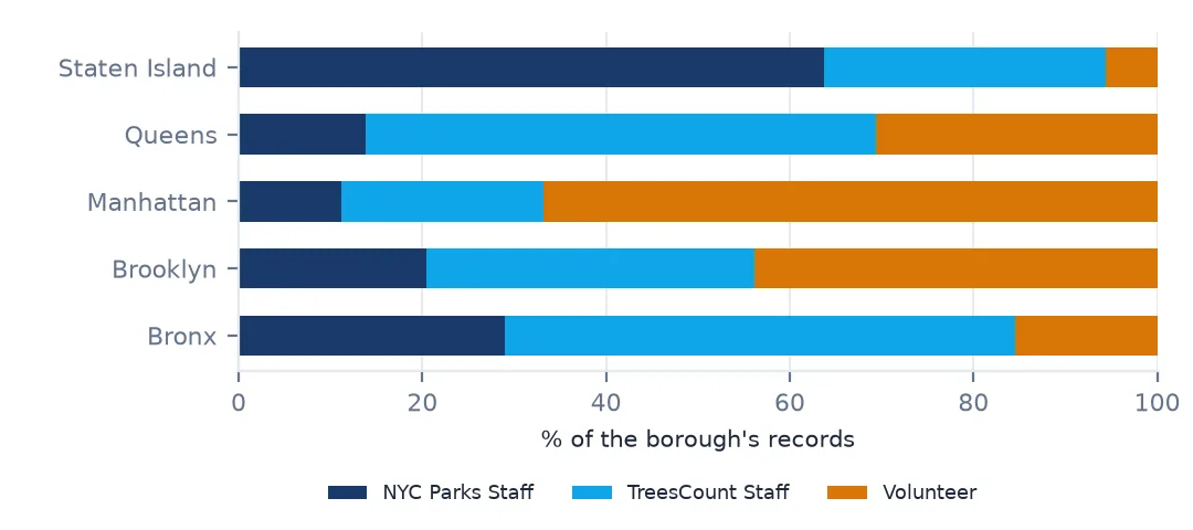
print(pd.crosstab(trees.borough, trees.user_type, normalize="index").round(3).to_string())
print("records per day, peak:", trees.created_at.value_counts().iloc[0], "on", trees.created_at.value_counts().index[0])

user_type      NYC Parks Staff  TreesCount Staff  Volunteer
borough                                                    
Bronx                    0.289             0.555      0.155
Brooklyn                 0.204             0.357      0.439
Manhattan                0.112             0.219      0.669
Queens                   0.138             0.555      0.307
Staten Island            0.637             0.307      0.057
records per day, peak: 6852 on 10/27/2015

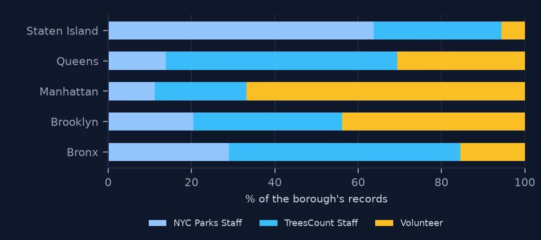
Who recorded the trees differs by borough: volunteers made 66.9% of Manhattan's records but 5.7% of Staten Island's, where city Parks staff made 63.7%. Any comparison between boroughs is also a comparison between recorders — volunteers and staff recorded trees differently tests how much that matters. The busiest day, 27 October 2015, added 6,852 records.

An inventory of places as well as trees

A street tree census is a record of the city's planting sites as much as of its trees. Every row is a location along a street, and status tells you what is there now: a living tree, a dead one waiting for removal, or a stump waiting for a replacement. That is why the file keeps all three, and why a "number of trees" depends on whether you count sites or living trees.

The other fields follow from how the survey was run. Teams walked every block with a protocol: identify the species, measure the trunk at breast height, judge the crown's health, tick the problems. The protocol makes the fields comparable across the city; the people — city staff, census staff, volunteers — make them slightly less so. The coordinates came from the survey's own mapping on the city's State Plane grid, and that grid is the safest base for anything measured on the ground.

Reading the census safely

• Read "None" as text for the guard, steward and problems fields: keep_default_na=False, or fill the missing values back with "None".
• Filter on status. Dead trees and stumps have no species or health.
• Coordinates are in feet in EPSG:2263; reproject before measuring.
• Diameters have impossible values at both ends.
• The nta codes are the 2010 neighbourhoods, not the 2020 ones (codes that match no boundary).

Internal links

• Street tree censuses explained — what each field records
• How to measure street tree species diversity by neighbourhood — the species field at work
• Street trees 425 inches across — the diameter column's errors
• Neighbourhood codes that match no boundary — joining trees to areas

FAQ

How many street trees are there in New York City?

The 2015 census recorded 652,173 living street trees, plus 17,654 stumps and 13,961 dead trees, 683,788 records in all.

What is the most common street tree in New York?

The London planetree: 13.3% of living street trees in the 2015 census, followed by the honeylocust and the Callery pear.