
How to Relate Street Tree Health to Sidewalk Damage and Site Conditions
On this page
Problem statement
Street trees and sidewalks fight: roots lift paving, and paving, stones and grates crowd roots. The 2015 New York tree census recorded both sides of that fight for every tree — whether the sidewalk was damaged, which problems affected roots, trunk and branches, and how healthy the tree looked. It is tempting to read the health of trees with damaged sidewalks straight off the table. But big trees break sidewalks and big trees are healthier, species differ in both, and recorders differ in what they tick.
This page relates tree health to sidewalk damage and site conditions with a model that holds size, species, borough and recorder fixed, and checks which site conditions still matter after that.
Quick answer
Fill the "None" guard values pandas reads as missing, turn the problem flags into 0/1, and fit a logistic model of fair-or-poor health with size, species, borough and recorder as controls; exponentiated coefficients are odds ratios:
import statsmodels.formula.api as smf

alive = trees[(trees.status == "Alive") & trees.health.notna()].copy()
alive["guards"] = alive.guards.fillna("None")                 # pandas reads the word "None" as missing
alive["unhealthy"] = alive.health.isin(["Fair", "Poor"]).astype(int)
flags = [c for c in alive.columns if c.startswith(("root_", "trunk_", "trnk_", "brch_"))]
for c in flags:
    alive[c] = (alive[c] == "Yes").astype(int)
alive["sidewalk_damage"] = (alive.sidewalk == "Damage").astype(int)
common = alive.spc_common.value_counts().index[:15]
d = alive[alive.spc_common.isin(common)]
fit = smf.logit("unhealthy ~ sidewalk_damage + root_stone + root_grate + trunk_wire + brch_light + brch_shoe"
                " + C(guards) + C(curb_loc) + np.log1p(tree_dbh) + C(spc_common) + C(borough) + C(user_type)", data=d).fit(disp=False)
odds = np.exp(fit.params[["sidewalk_damage", "root_stone", "root_grate", "trunk_wire", "brch_light", "brch_shoe"]])
print(odds.round(2).to_string())
print(f"n = {int(fit.nobs):,}")
sidewalk_damage 1.01
root_stone 1.28
root_grate 1.68
trunk_wire 1.49
brch_light 1.20
brch_shoe 2.12
n = 496,183
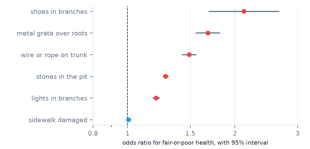
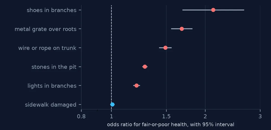
Holding the controls fixed, a damaged sidewalk is unrelated to tree health (odds ratio 1.01). The conditions that matter are the ones that wound the tree: shoes thrown over branches (2.12), metal grates over the roots (1.68), wire or rope around the trunk (1.49), stones in the pit (1.28) and lights in the branches (1.20). The model uses all 496,183 trees of the 15 commonest species.
Raw rates, size, species and site
1. Raw rates first
for c in ["sidewalk_damage", "root_stone", "brch_shoe", "trunk_wire"]:
    r = alive.groupby(c).unhealthy.mean()
    print(f"{c:16s} fair-or-poor: without {r.loc[0]:.1%}, with {r.loc[1]:.1%}   (flagged on {alive[c].mean():.1%})")
sidewalk_damage fair-or-poor: without 18.9%, with 18.9% (flagged on 28.7%)
root_stone fair-or-poor: without 18.5%, with 20.5% (flagged on 21.5%)
brch_shoe fair-or-poor: without 18.9%, with 30.7% (flagged on 0.1%)
trunk_wire fair-or-poor: without 18.8%, with 26.5% (flagged on 2.0%)
In the raw data, 18.9% of trees are in fair or poor health with or without sidewalk damage, which is flagged on 28.7% of trees. Trunk wires and branch shoes are rare — on 2.0% and 0.1% of trees — but trees with them are much more often unhealthy (26.5% and 30.7%).
2. Big trees break sidewalks
size = pd.cut(alive.tree_dbh, [0, 6, 12, 18, 24, 500], labels=["<6", "6-12", "12-18", "18-24", "24+"])
print(alive.groupby(size, observed=True)[["sidewalk_damage", "unhealthy"]].mean().round(3).to_string())
sidewalk_damage unhealthy
tree_dbh
<6 0.154 0.209
6-12 0.281 0.196
12-18 0.391 0.190
18-24 0.420 0.167
24+ 0.460 0.117
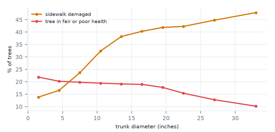
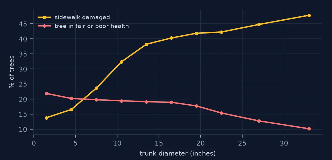
Size explains why sidewalk damage looks harmless or even protective: damage rises from 15.4% of trees under 6 inches to 46.0% of trees over 24, while the share in fair or poor health falls from 20.9% to 11.7%. Large trees break sidewalks and large trees have survived; without controlling for size, damage would appear to make trees healthier.
3. Species differ in both
sp = alive[alive.spc_common.isin(common)].groupby("spc_common")[["sidewalk_damage", "unhealthy"]].mean()
print(sp.sort_values("sidewalk_damage").round(3).iloc[[0, 1, -2, -1]].to_string())
sidewalk_damage unhealthy
spc_common
cherry 0.145 0.162
Callery pear 0.218 0.184
silver maple 0.382 0.229
London planetree 0.396 0.157
Species differ in both: London planetrees damage 39.6% of their sidewalks and are 15.7% unhealthy, silver maples 38.2% and 22.9%; cherries damage few sidewalks (14.5%). Species is therefore a confounder too.
4. Guards and curb position
print(alive.groupby("guards").unhealthy.agg(["mean", "size"]).round(3).to_string())
print(alive.groupby("curb_loc").unhealthy.agg(["mean", "size"]).round(3).to_string())
mean size
guards
Harmful 0.243 20252
Helpful 0.178 51866
None 0.188 572306
Unsure 0.237 7748
mean size
curb_loc
OffsetFromCurb 0.193 25875
OnCurb 0.189 626297
Guards rated "Harmful" go with more unhealthy trees (24.3%) than "Helpful" ones (17.8%) or none (18.8%). Whether a tree stands on the curb or set back from it makes no difference (18.9% against 19.3%).
Neighbourhoods and fit
The data used on this page
New York City Department of Parks and Recreation, TreesCount! 2015 Street Tree Census on NYC Open Data: one row for every street tree, stump and dead tree mapped by staff and volunteers in 2015–2016, with species, trunk diameter, health and site conditions.
from pathlib import Path

import numpy as np
import pandas as pd
import requests

Path("data").mkdir(exist_ok=True)
SOCRATA = "https://data.cityofnewyork.us/api/views/{}/rows.csv?accessType=DOWNLOAD"
f = Path("data/nyc-street-tree-census-2015.csv")
if not f.exists():
    # TreesCount! 2015, the finished census (220 MB), NYC Open Data dataset uvpi-gqnh
    f.write_bytes(requests.get(SOCRATA.format("uvpi-gqnh"), timeout=1800).content)
trees = pd.read_csv(f, low_memory=False)
print(f"{len(trees):,} trees, {trees.status.eq('Alive').sum():,} alive")
683,788 trees, 652,173 alive
Example 1: neighbourhood rates after adjustment
d = d.assign(pred=fit.predict(d))
nta = d.groupby("nta_name").agg(trees=("tree_id", "size"), observed=("unhealthy", "mean"), expected=("pred", "mean"))
nta = nta[nta.trees >= 500]
nta["ratio"] = nta.observed / nta.expected
print(nta.sort_values("ratio").round(2).iloc[[0, 1, -2, -1]].to_string())
trees observed expected ratio
nta_name
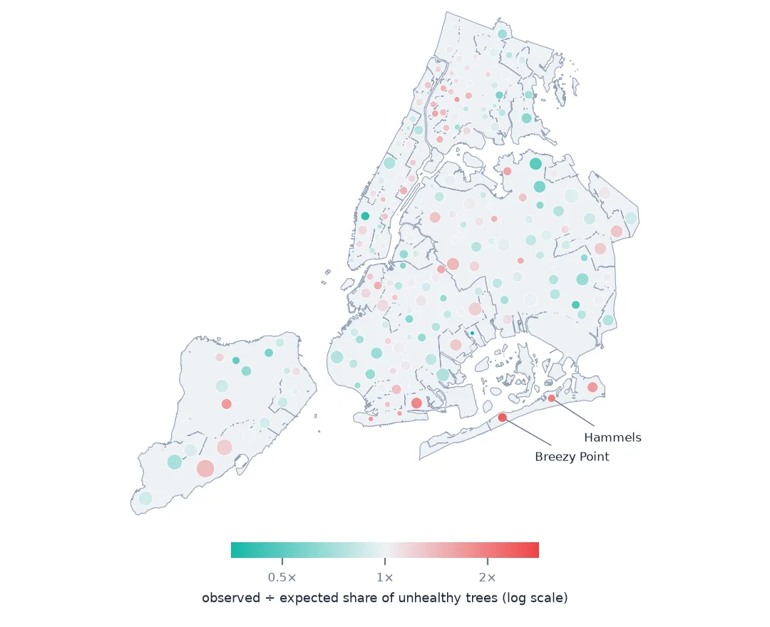
Starrett City 578 0.05 0.16 0.33
Hudson Yards-Chelsea-Flatiron-Union Square 2426 0.09 0.24 0.40
Hammels-Arverne-Edgemere 1973 0.38 0.19 2.01
Breezy Point-Belle Harbor-Rockaway Park-Broad Channel 2729 0.43 0.18 2.41
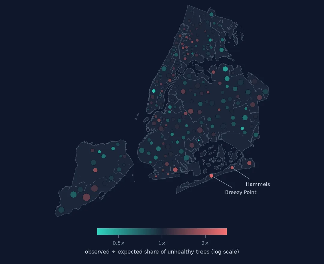
Comparing each neighbourhood's observed share of unhealthy trees with the model's expectation picks out places the site conditions do not explain. The two highest ratios are both on the Rockaway peninsula — Breezy Point–Belle Harbor (2.41 times the expected share) and Hammels–Arverne–Edgemere (2.01) — the area most flooded by seawater in Hurricane Sandy in 2012; the census cannot confirm the cause, but the model points to it. Starrett City's trees are healthier than expected (0.33).
Example 2: the model's fit
from sklearn.metrics import roc_auc_score
ok = d.pred.notna()
print(f"AUC {roc_auc_score(d.unhealthy[ok], d.pred[ok]):.3f}; pseudo R² {fit.prsquared:.3f}; rows used {ok.sum():,} of {len(d):,}")
AUC 0.631; pseudo R² 0.037; rows used 496,183 of 496,183
The model discriminates weakly (AUC 0.631, pseudo R² 0.037): site conditions, size, species and place explain little of why one tree is rated fair and its neighbour good. Health is mostly individual — and partly the judgement of the person rating it.
Confounding on the sidewalk
The sidewalk result is a textbook case of confounding. Damage and health are both driven by tree size: roots grow with the tree, and trees that reach a large size are the survivors. A raw comparison shows no association, a size table shows the two moving in opposite directions, and only a model that holds size and species fixed can ask whether, among similar trees, damage goes with poorer health. It does not.
The conditions that remain are wounds and constraints: objects that cut or girdle the trunk and branches, grates that limit the root zone, stones that compact it. They are also the cheapest to fix, which makes the model useful for maintenance even though it explains little of the variation. A model of tree health from a census is a screening tool, not a forecast; its value is in what it rules out and in the places whose trees are worse than their conditions predict.
Pitfalls in tree-health models
- Control for size. It drives both damage and survival.
- Control for species and recorder; both affect health ratings.
- "None" guards are values. Leaving them as NaN drops most rows from the model.
- Rare flags have wide intervals. Branch shoes are on 0.1% of trees.
- Low AUC is normal for individual health; use the model for comparison, not prediction.
Internal links
- Volunteers and staff recorded trees differently — why recorder type is in the model
- Street tree censuses explained — the condition fields
- How to measure street tree species diversity — species by neighbourhood
FAQ
Does sidewalk damage harm street trees?
In New York's 2015 census, not once tree size, species, borough and recorder are held fixed: the odds ratio for fair-or-poor health was 1.01. Wounds such as shoes in branches (2.12) and wires on trunks (1.49) mattered more.
Why do bigger street trees damage more sidewalks?
Roots grow with the tree: 46.0% of trees over 24 inches had sidewalk damage, against 15.4% under 6 inches.