Volunteers and Staff Recorded Trees Differently: Measurer Bias in Citizen Data

Problem statement

A third of New York's 2015 street tree census was recorded by volunteers, the rest by census staff and Parks Department foresters. When a dataset mixes trained and untrained recorders, every field that needs judgement — is this tree in fair or poor health, are those roots damaging the sidewalk — may carry the recorder's habits as well as the tree's condition. A map of tree health could then partly be a map of who did the survey.

Testing for that is harder than comparing averages, because the recorders did not survey the same places. This page compares them first naively, then within the same census tracts and with species and size held fixed, field by field, and finds which fields are affected and which are not.

Quick answer

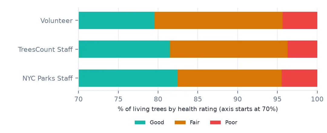
The naive comparison — health and size by recorder type across all trees:

alive = trees[trees.status == "Alive"].copy()
print(pd.crosstab(alive.user_type, alive.health, normalize="index").round(3).to_string())
print(alive.groupby("user_type").tree_dbh.median().to_string())

health             Fair   Good   Poor
user_type                            
NYC Parks Staff   0.131  0.824  0.045
TreesCount Staff  0.148  0.815  0.037
Volunteer         0.161  0.795  0.044
user_type
NYC Parks Staff     10.0
TreesCount Staff    10.0
Volunteer           10.0

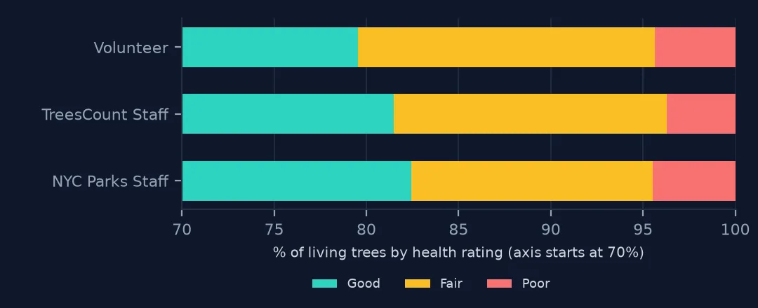
Volunteers rated 16.1% of trees Fair against 13.1% for Parks staff and 14.8% for census staff; the median diameter is 10 inches for all three. The gap is small, and as the next steps show, part of it is place, not people.

Separating recorders from places

1. They did not survey the same places

print(pd.crosstab(alive.borough, alive.user_type, normalize="columns").round(3).to_string())

user_type      NYC Parks Staff  TreesCount Staff  Volunteer
borough                                                    
Bronx                    0.141             0.160      0.060
Brooklyn                 0.213             0.215      0.359
Manhattan                0.043             0.049      0.201
Queens                   0.203             0.467      0.352
Staten Island            0.400             0.109      0.027

The recorders covered different parts of the city: 40.0% of Parks staff records are on Staten Island, against 2.7% of volunteer records; volunteers worked mostly in Brooklyn (35.9%), Queens (35.2%) and Manhattan (20.1%). Any raw difference between recorder groups is also a difference between boroughs, species mixes and street types.

2. Every block had one recorder

blk = alive.groupby("block_id").user_type.nunique()
print(f"blocks surveyed by more than one kind of recorder: {(blk > 1).sum():,} of {len(blk):,}")
tr = alive.groupby("boro_ct").user_type.nunique()
mixed = alive[alive.boro_ct.isin(tr[tr > 1].index)].assign(fair_or_poor=lambda d: d.health.isin(["Fair", "Poor"]))
print(f"census tracts with more than one kind of recorder: {(tr > 1).sum():,} of {len(tr):,}; trees in them {len(mixed):,}")
cell = mixed.groupby(["boro_ct", "user_type"]).fair_or_poor.mean().unstack()
for other in ["NYC Parks Staff", "Volunteer"]:
    diff = (cell[other] - cell["TreesCount Staff"]).dropna()
    print(f"{other} minus TreesCount Staff, fair-or-poor share within the same tract: median {diff.median():+.3f} over {len(diff):,} tracts")

blocks surveyed by more than one kind of recorder: 0 of 100,700
census tracts with more than one kind of recorder: 1,829 of 2,152; trees in them 578,176
NYC Parks Staff minus TreesCount Staff, fair-or-poor share within the same tract: median -0.017 over 1,073 tracts
Volunteer minus TreesCount Staff, fair-or-poor share within the same tract: median +0.008 over 1,411 tracts

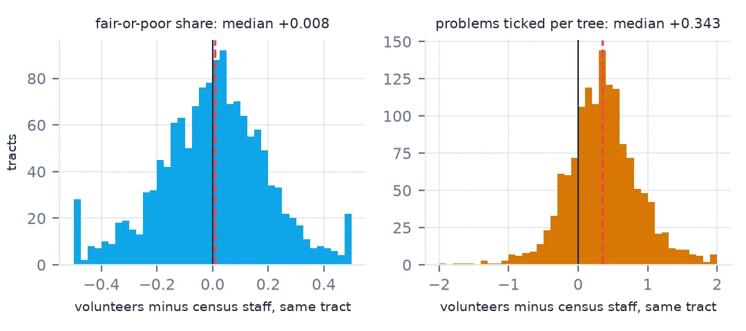
The survey assigned each block to one team: not one of 100,700 blocks was recorded by more than one kind of recorder, so a same-block comparison is impossible. Census tracts are mixed — 1,829 of 2,152 contain more than one kind — and comparing recorders within a tract holds the neighbourhood roughly fixed. Within the same tract, volunteers rated a median 0.008 more of their trees fair or poor than census staff, and Parks staff 0.017 fewer: differences of about a percentage point.

3. Problems ticked

flags = [c for c in alive.columns if c.startswith(("root_", "trunk_", "trnk_", "brch_"))]
mixed["n_problems"] = (mixed[flags] == "Yes").sum(axis=1)
mixed["sidewalk_damage"] = mixed.sidewalk == "Damage"
cell2 = mixed.groupby(["boro_ct", "user_type"])[["n_problems", "sidewalk_damage"]].mean()
for col in ["n_problems", "sidewalk_damage"]:
    u = cell2[col].unstack()
    print(col, {o: round(float((u[o] - u["TreesCount Staff"]).dropna().median()), 3) for o in ["NYC Parks Staff", "Volunteer"]})

n_problems {'NYC Parks Staff': 0.008, 'Volunteer': 0.343}
sidewalk_damage {'NYC Parks Staff': -0.008, 'Volunteer': 0.068}

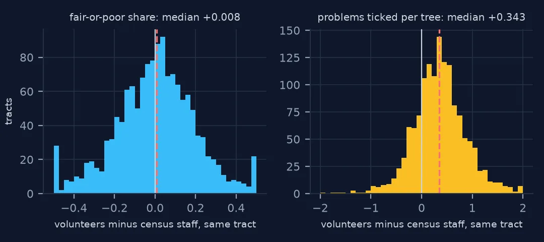
The problem checklist is a different story. Within the same tract, volunteers ticked a median 0.343 more problems per tree than census staff and recorded sidewalk damage on a 0.068 larger share of trees; Parks staff were within a point of census staff on both. Volunteers looked harder, or counted more generously, at the things a checklist asks about.

4. Rounding of diameters

mid = alive[alive.tree_dbh.between(5, 40)]
print(mid.groupby("user_type").tree_dbh.apply(lambda s: (s % 5 == 0).mean()).round(3).to_dict(), "(0.2 if no rounding)")
print(mid.groupby("user_type").tree_dbh.apply(lambda s: (s % 2 == 0).mean()).round(3).to_dict(), "(0.5 if no rounding)")

{'NYC Parks Staff': 0.238, 'TreesCount Staff': 0.235, 'Volunteer': 0.238} (0.2 if no rounding)
{'NYC Parks Staff': 0.478, 'TreesCount Staff': 0.475, 'Volunteer': 0.472} (0.5 if no rounding)

Diameter rounding is the same for all three groups — a share of 0.235–0.238 of values on a multiple of five and 0.472–0.478 even — so the tape measurements are as good from volunteers as from staff.

A model and a map

The data used on this page

New York City Department of Parks and Recreation, TreesCount! 2015 Street Tree Census on NYC Open Data: one row for every street tree, stump and dead tree mapped by staff and volunteers in 2015–2016, with species, trunk diameter, health and site conditions.

from pathlib import Path

import numpy as np
import pandas as pd
import requests

Path("data").mkdir(exist_ok=True)
SOCRATA = "https://data.cityofnewyork.us/api/views/{}/rows.csv?accessType=DOWNLOAD"
f = Path("data/nyc-street-tree-census-2015.csv")
if not f.exists():
    # TreesCount! 2015, the finished census (220 MB), NYC Open Data dataset uvpi-gqnh
    f.write_bytes(requests.get(SOCRATA.format("uvpi-gqnh"), timeout=1800).content)
trees = pd.read_csv(f, low_memory=False)
print(f"{len(trees):,} trees, {trees.status.eq('Alive').sum():,} alive")

683,788 trees, 652,173 alive

Example 1: a model with recorder, species, size and tract

d = mixed[mixed.spc_common.isin(mixed.spc_common.value_counts().index[:10])].copy()
X = pd.get_dummies(d[["spc_common"]], drop_first=True, dtype=float)
X[["parks_staff", "volunteer"]] = pd.get_dummies(d.user_type, dtype=float)[["NYC Parks Staff", "Volunteer"]].values
X["log_dbh"] = np.log1p(d.tree_dbh)
y = d.fair_or_poor.astype(float)
Xd = X - X.groupby(d.boro_ct.values).transform("mean")          # within-tract: compare like places only
yd = y - y.groupby(d.boro_ct.values).transform("mean")
beta = pd.Series(np.linalg.lstsq(Xd.values, yd.values, rcond=None)[0], index=X.columns)
print((100 * beta[["parks_staff", "volunteer"]]).round(2).to_string(), "percentage points against TreesCount Staff")
print(f"n = {len(d):,} trees in {d.boro_ct.nunique():,} tracts")

parks_staff   -1.49
volunteer      0.15 percentage points against TreesCount Staff
n = 376,111 trees in 1,828 tracts

Holding tract, species and size fixed together with a within-tract regression on 376,111 trees, volunteers' fair-or-poor share is 0.15 percentage points above census staff — no measurable effect — and Parks staff's 1.49 points below. The health ratings are consistent across recorders once place and tree are accounted for.

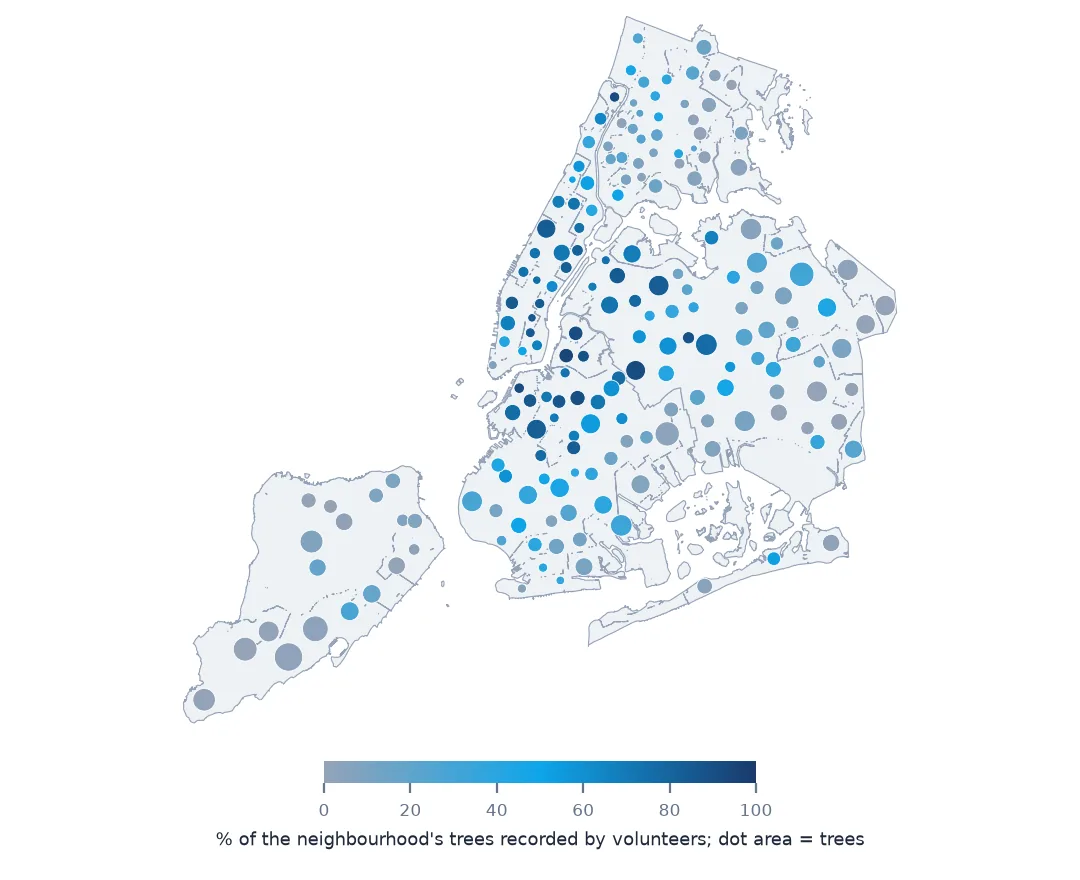
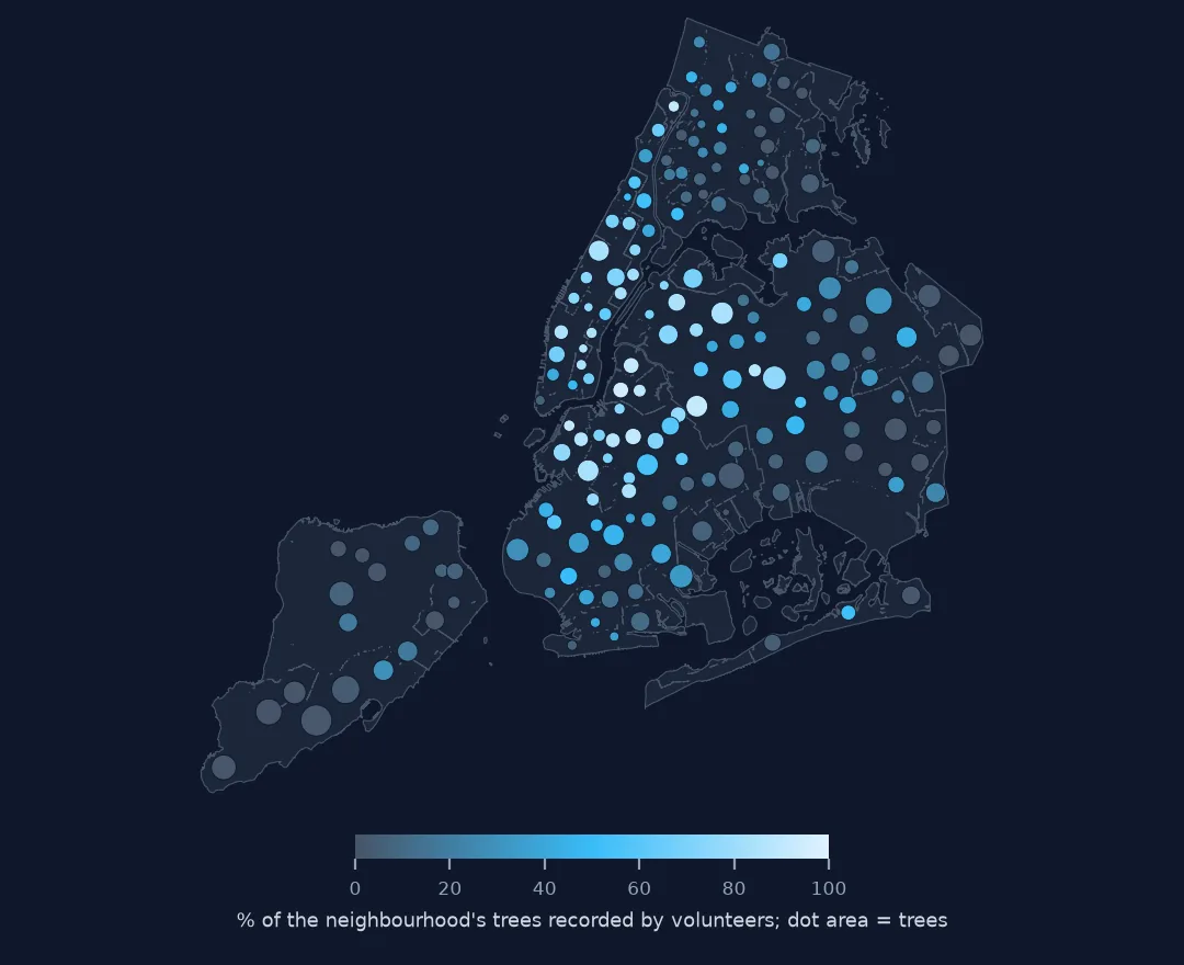
Example 2: what a naive map would show

vol = alive.groupby("nta_name").agg(trees=("tree_id", "size"), volunteer=("user_type", lambda s: (s == "Volunteer").mean()),
                                    fair_or_poor=("health", lambda s: s.isin(["Fair", "Poor"]).mean()))
vol = vol[vol.trees >= 500]
print(f"correlation across neighbourhoods of volunteer share and fair-or-poor share: {vol.volunteer.corr(vol.fair_or_poor, method='spearman'):.2f}")

correlation across neighbourhoods of volunteer share and fair-or-poor share: 0.31

Without that adjustment, a map would mislead: across neighbourhoods, the share of trees recorded by volunteers correlates at 0.31 with the share rated fair or poor. Neighbourhoods surveyed by volunteers look less healthy, largely because volunteers were assigned to different neighbourhoods, not because they rated differently.

Testing for a measurer effect

A recorder effect can only be separated from a place effect where recorders overlap. Here the survey design made overlap impossible at the block level and common at the tract level, so the tract is the finest place that can be held fixed. A within-tract comparison asks whether, in the same neighbourhood, one group rated differently — and the answer depends on the field. Health ratings agree within about a point; the problem checklist does not.

That pattern is typical of citizen science. Simple, trained judgements with few categories transfer well from staff to volunteers; long checklists of conditions, where noticing is part of the task, do not. The practical response is not to discard volunteer data but to keep user_type in every analysis of judgement fields, and to report findings that depend on checklists with and without it.

Pitfalls with mixed-recorder data

• Recorders cover different places. Raw differences are mostly place.
• Hold place fixed where recorders overlap — here tracts, not blocks.
• Judgement fields differ more than measurements. Checklists were affected, diameters were not.
• Maps of judgement fields can show who surveyed where.
• Keep user_type in models of health and problems.

Internal links

• Street trees 425 inches across — the diameter errors
• Street tree censuses explained — who recorded what
• How to relate street tree health to sidewalk damage — the health field modelled
• Annual average daily flow explained — another survey with recorder effects designed out

FAQ

Are volunteer tree census data reliable?

For diameter and health in New York's 2015 census, yes: within the same census tracts and holding species and size fixed, volunteers' health ratings were within 0.15 percentage points of census staff's. For the problem checklist they ticked 0.343 more problems per tree.

How do I test for observer bias in survey data?

Compare observers within units they both covered — here census tracts — and adjust for what differs between them, such as species and size.