
How to Compare Two Street Tree Censuses: New York 2005 and 2015
On this page
Problem statement
New York counted its street trees in 2005 and again in 2015, so the obvious question is what changed: how many trees were gained or lost, which species were planted and which declined, and where. The two files look alike, but they were made with different protocols, different health classes, different species names and, it turns out, different ways of placing a tree on the map. A careless comparison mixes all of those into the "change".
This page compares the two censuses at the levels where they can be compared — boroughs, species once names are reconciled, size classes and a 1-km grid — and shows why individual trees cannot be followed from one to the other.
Quick answer
Fix the 2005 file's borough codes, define "living" in each census by its own status field, and compare counts by borough:
old = pd.read_csv(f05, low_memory=False, usecols=["status", "spc_common", "tree_dbh", "boroname", "x_sp", "y_sp"])
old["borough"] = old.boroname.replace({"5": "Staten Island"})
old_alive = old[old.status != "Dead"]
new_alive = trees[trees.status == "Alive"]
cmp = pd.DataFrame({"2005": old_alive.borough.value_counts(), "2015": new_alive.borough.value_counts()})
cmp["change"] = cmp["2015"] / cmp["2005"] - 1
print(cmp.assign(change=(100 * cmp.change).round(1)).to_string())
print(f"city: {len(old_alive):,} living trees in 2005, {len(new_alive):,} in 2015 ({len(new_alive) / len(old_alive) - 1:+.1%})")
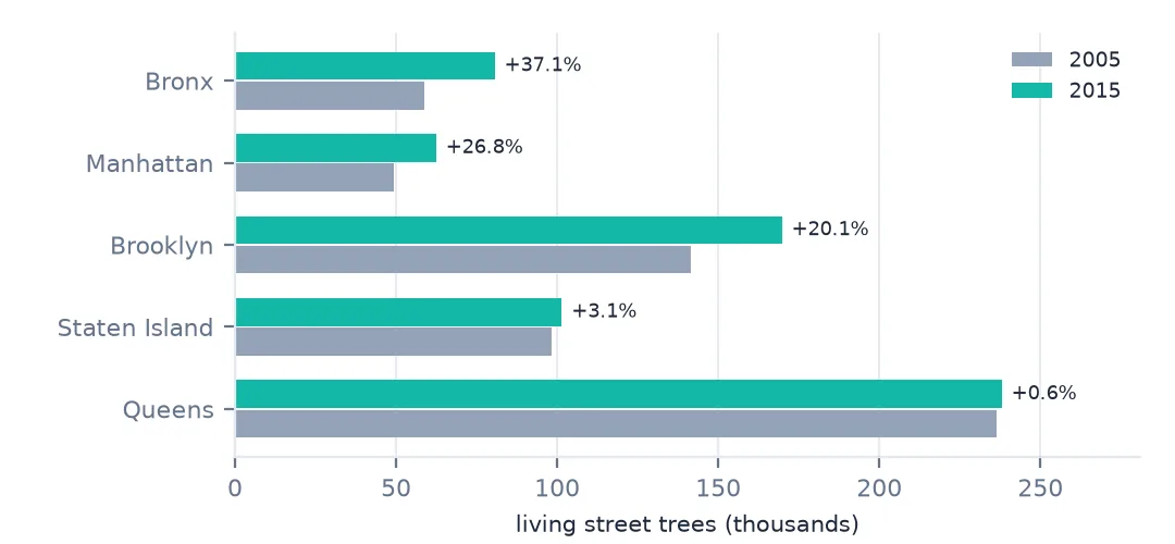
2005 2015 change
borough
Queens 236523 237974 0.6
Brooklyn 141322 169744 20.1
Staten Island 98425 101443 3.1
Bronx 58759 80585 37.1
Manhattan 49223 62427 26.8
city: 584,252 living trees in 2005, 652,173 in 2015 (+11.6%)
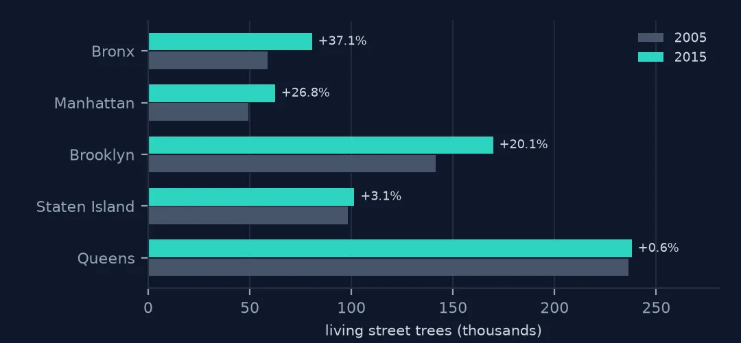
The city had 584,252 living street trees in 2005 and 652,173 in 2015, 11.6% more. The growth was uneven: the Bronx gained 37.1%, Manhattan 26.8% and Brooklyn 20.1%, while Queens, already the most planted, gained 0.6% and Staten Island 3.1%.
Reconciling two censuses
1. Make the two files speak the same language
print("2005 borough values:", old.boroname.value_counts().to_dict())
print("2005 status:", old.status.value_counts().to_dict())
print("2015 status and health:", trees.status.value_counts().to_dict(), trees.health.value_counts().to_dict())
2005 borough values: {'Queens': 240008, 'Brooklyn': 142852, '5': 99701, 'Bronx': 59925, 'Manhattan': 49886}
2005 status: {'Good': 393464, 'Excellent': 141657, 'Poor': 49131, 'Dead': 8120}
2015 status and health: {'Alive': 652173, 'Stump': 17654, 'Dead': 13961} {'Good': 528850, 'Fair': 96504, 'Poor': 26818}
Staten Island is coded "5" in the 2005 file instead of a name, and health and death share one field: Excellent, Good, Poor or Dead. In 2015, status (Alive, Stump, Dead) and health (Good, Fair, Poor) are separate. Health classes cannot be compared across the two files, so this page compares living trees only.
2. Species names changed too
a, b = set(old_alive.spc_common.dropna().str.lower()), set(new_alive.spc_common.dropna().str.lower())
print(f"species names: {len(a)} in 2005, {len(b)} in 2015, {len(a & b)} in both")
print("examples only in 2005:", sorted(a - b)[:8])
print("examples only in 2015:", sorted(b - a)[:8])
species names: 168 in 2005, 132 in 2015, 23 in both
examples only in 2005: ['alder, european', 'american smoketree', 'amur corktree', 'apple', 'arborvitae, eastern', 'ash, green', 'ash, other', 'ash, white']
examples only in 2015: ["'schubert' chokecherry", 'american beech', 'american elm', 'american hophornbeam', 'american hornbeam', 'american larch', 'american linden', 'amur cork tree']
Lower-cased, only 23 species names appear in both files. The 2005 census wrote names genus-first with a comma — "ash, green" — and the 2015 census as they are spoken — "green ash".
3. Compare species that can be matched
def norm(s):
    s = s.str.lower().str.replace(r"^([^,]+),\s*(.+)$", r"\2 \1", regex=True)     # "ash, green" -> "green ash"
    return s.str.replace(r"[^a-z]", "", regex=True)
o = norm(old_alive.spc_common).value_counts(); n = norm(new_alive.spc_common).value_counts()
sp = pd.DataFrame({"2005": o, "2015": n}).dropna()
print(f"species matched after reordering: {len(sp)} of {len(o)} (2005) and {len(n)} (2015)")
sp["change"] = sp["2015"] / sp["2005"] - 1
big = sp[sp["2005"] >= 5000].sort_values("change")
print(big.assign(change=(100 * big.change).round(0)).astype({"2005": int, "2015": int}).to_string())
species matched after reordering: 91 of 168 (2005) and 132 (2015)
2005 2015 change
spc_common
norwaymaple 74007 34189 -54.0
silvermaple 18624 12277 -34.0
northernredoak 11037 8400 -24.0
greenash 20555 16251 -21.0
redmaple 20148 17246 -14.0
callerypear 63388 58931 -7.0
londonplanetree 89362 87014 -3.0
littleleaflinden 27491 29742 8.0
pinoak 43790 53185 21.0
honeylocust 52062 64263 23.0
sweetgum 8365 10657 27.0
ginkgo 16186 21024 30.0
silverlinden 5991 7995 33.0
americanelm 5452 7975 46.0
americanlinden 7187 13530 88.0
japanesezelkova 14556 29258 101.0
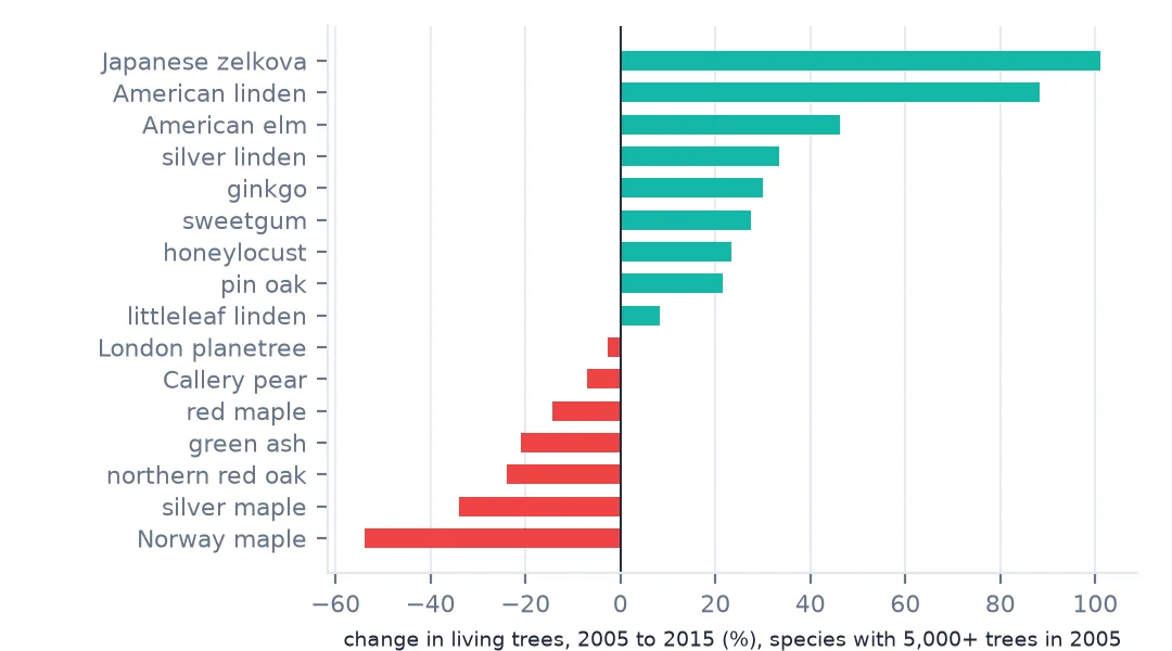
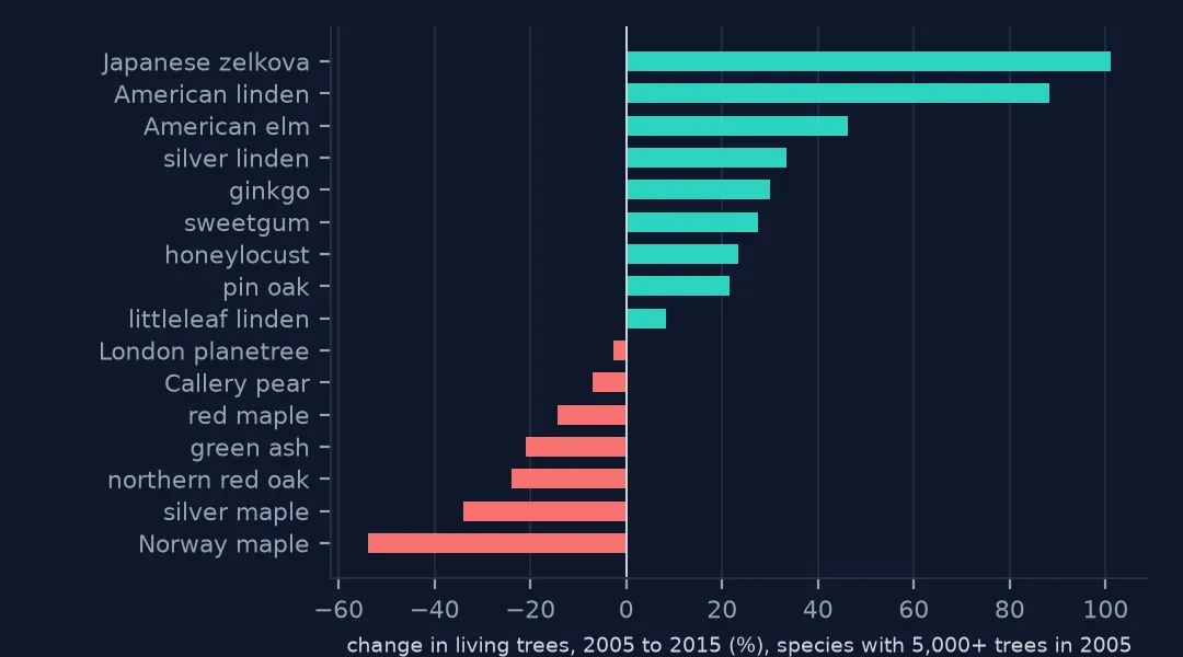
Reordering "ash, green" to "green ash" and stripping punctuation matches 91 species. Among the common species, the Norway maple fell by 54%, silver maple by 34%, red oak and green ash by around a fifth; Japanese zelkova doubled, American linden grew 88% and American elm 46%.
4. Change on a grid, not by name
cell = 1000 * 3.28084                                         # 1 km in US survey feet
gx = lambda df: (df.x_sp // cell).astype(int).astype(str) + "_" + (df.y_sp // cell).astype(int).astype(str)
grid = pd.DataFrame({"2005": gx(old_alive).value_counts(), "2015": gx(new_alive).value_counts()}).fillna(0)
grid = grid[(grid["2005"] + grid["2015"]) >= 100]
grid["change"] = grid["2015"] - grid["2005"]
print(f"{len(grid):,} 1-km cells; median change {grid.change.median():+.0f} trees; cells that lost trees: {(grid.change < 0).mean():.0%}")
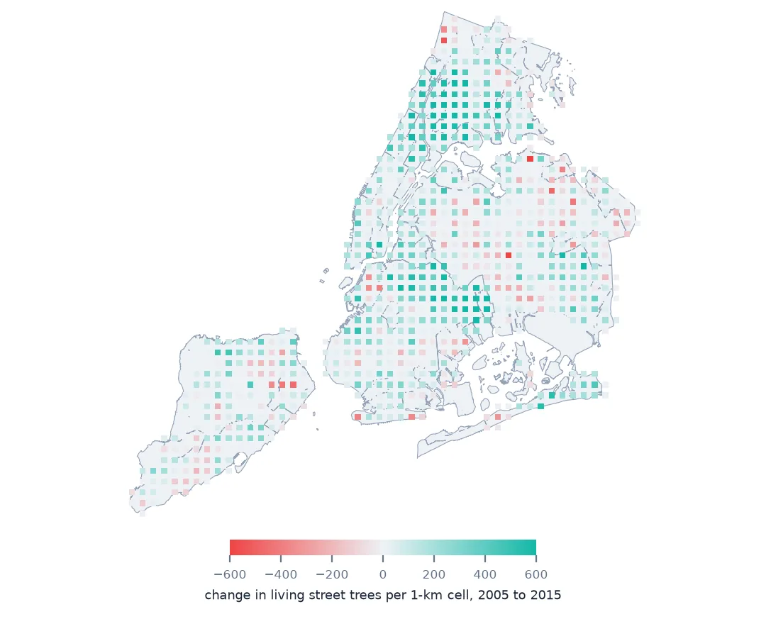
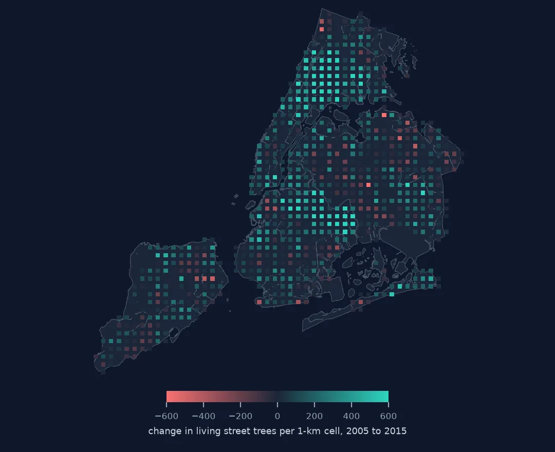
777 1-km cells; median change +82 trees; cells that lost trees: 30%
On a 1-km grid, using each census's own coordinates, the median cell gained 82 trees and 30% of cells lost trees. A grid is coarse enough to absorb the different ways the two censuses placed trees, which the next example shows matters.
Size classes and the locations
The data used on this page
New York City Department of Parks and Recreation, TreesCount! 2015 Street Tree Census on NYC Open Data: one row for every street tree, stump and dead tree mapped by staff and volunteers in 2015–2016, with species, trunk diameter, health and site conditions. The 2005 census is NYC Open Data dataset 29bw-z7pj.
from pathlib import Path

import numpy as np
import pandas as pd
import requests

Path("data").mkdir(exist_ok=True)
SOCRATA = "https://data.cityofnewyork.us/api/views/{}/rows.csv?accessType=DOWNLOAD"
f = Path("data/nyc-street-tree-census-2015.csv")
if not f.exists():
    # TreesCount! 2015, the finished census (220 MB), NYC Open Data dataset uvpi-gqnh
    f.write_bytes(requests.get(SOCRATA.format("uvpi-gqnh"), timeout=1800).content)
f05 = Path("data/nyc-street-tree-census-2005.csv")
if not f05.exists():
    # the 2005 census (204 MB), NYC Open Data dataset 29bw-z7pj
    f05.write_bytes(requests.get(SOCRATA.format("29bw-z7pj"), timeout=1800).content)
trees = pd.read_csv(f, low_memory=False)
print(f"{len(trees):,} trees, {trees.status.eq('Alive').sum():,} alive")
683,788 trees, 652,173 alive
Example 1: the size structure shifted
bins = [0, 3, 6, 12, 18, 24, 500]
dist = pd.DataFrame({"2005": pd.cut(old_alive.tree_dbh, bins).value_counts(normalize=True, sort=False),
                     "2015": pd.cut(new_alive.tree_dbh, bins).value_counts(normalize=True, sort=False)})
print((100 * dist).round(1).to_string())
2005 2015
tree_dbh
(0, 3] 10.4 14.2
(3, 6] 18.0 20.7
(6, 12] 29.7 27.9
(12, 18] 18.6 18.1
(18, 24] 11.9 9.6
(24, 500] 11.4 9.6
Trees of 3 inches or less rose from 10.4% to 14.2% of the population and trees over 24 inches fell from 11.4% to 9.6%: a younger forest.
Example 2: no tree can be followed from one census to the next
print("shared id columns:", sorted(set(old.columns) & {"tree_id", "OBJECTID", "objectid"}), "against", [c for c in trees.columns if "id" in c])
o_xy = np.c_[old_alive.x_sp, old_alive.y_sp]; n_xy = np.c_[new_alive.x_sp, new_alive.y_sp]
from scipy.spatial import cKDTree
dist_ft, _ = cKDTree(o_xy).query(n_xy)
print(f"2015 trees within 3 m (9.8 ft) of a 2005 tree: {(dist_ft < 9.84).mean():.1%}; median distance {np.median(dist_ft) * 0.3048:.0f} m")
self_d, _ = cKDTree(o_xy).query(o_xy, k=2)
print(f"2005 trees sharing their exact coordinates with another 2005 tree: {(self_d[:, 1] == 0).mean():.1%}")
shared id columns: [] against ['tree_id', 'block_id', 'sidewalk']
2015 trees within 3 m (9.8 ft) of a 2005 tree: 0.5%; median distance 16 m
2005 trees sharing their exact coordinates with another 2005 tree: 73.9%
There is no shared id, so trees cannot be linked by key — and not by location either. Only 0.5% of 2015 trees are within 3 m of a 2005 tree, and the median distance is 16 m, much more than the trees' own spacing. The reason is in the 2005 coordinates: 73.9% of 2005 trees share their exact coordinates with another tree. The 2005 census appears to have placed trees at their street address, stacking the trees in front of a building on one point; the 2015 census mapped each tree where it stands. Tree-by-tree survival or growth cannot be measured from these two files.
Comparing surveys, not trees
Two censuses of the same thing are only as comparable as their methods. Here the methods differ in four ways: what counts as alive, how health is graded, how species are named, and how locations are recorded. Each difference has a remedy at some level of aggregation — status recoded to living trees, names reconciled, sizes binned, locations gridded — and no remedy at the level of the individual tree.
That limits the questions. "How many more trees, where, of which species and sizes?" can be answered. "Which trees died, and how fast did the survivors grow?" cannot, without a linked panel of individually tagged trees, which New York did not build between these two surveys. The planting record (the city's work orders) would add the missing link for new trees, and is the right next dataset for anyone studying survival.
Traps in census comparisons
- Staten Island is "5" in 2005. Recode before grouping.
- Health classes differ. Compare living trees, not health.
- Species names are written differently. Reorder "genus, species" names before matching.
- 2005 locations are addresses, stacked on one point per building.
- No tree can be linked between the censuses.
Internal links
- Street tree censuses explained — what each census recorded
- How to measure street tree species diversity by neighbourhood — the 2015 species mix
- How to analyse New York's street tree census — the 2015 file
- How to measure traffic trends from count points that were actually counted — comparing surveys over time elsewhere
FAQ
How much did New York's street tree count change between 2005 and 2015?
From 584,252 living street trees to 652,173, an 11.6% increase, with the largest gains in the Bronx (37.1%) and Manhattan (26.8%).
Can I track individual trees between the 2005 and 2015 NYC tree censuses?
No. There is no shared id, and 73.9% of 2005 trees were placed at shared address points rather than at the tree.