How to Build Desire Lines from Origin–Destination Data in Python

On this page

Problem statement

A desire line is a straight line from where a trip starts to where it wants to end, regardless of the roads in between. Transport planners use them to see demand before it is squeezed onto a network: where a new bus route or bike lane would serve the most trips. In GIS terms a set of desire lines is an ordinary line layer. Each line carries its origin, destination and count, so it can be filtered, buffered, intersected and saved like any other layer. Building one from an OD table means choosing the zones and the point each line starts from. It also means deciding which pairs are worth a line, because a few thousand thin lines hide the dozens that matter.

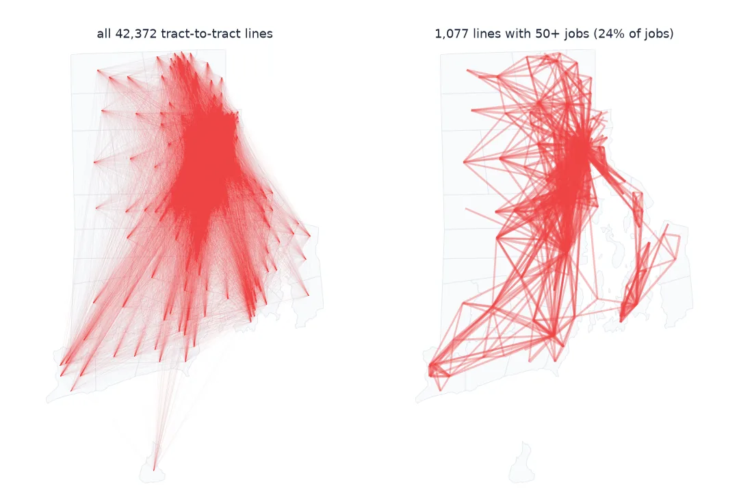
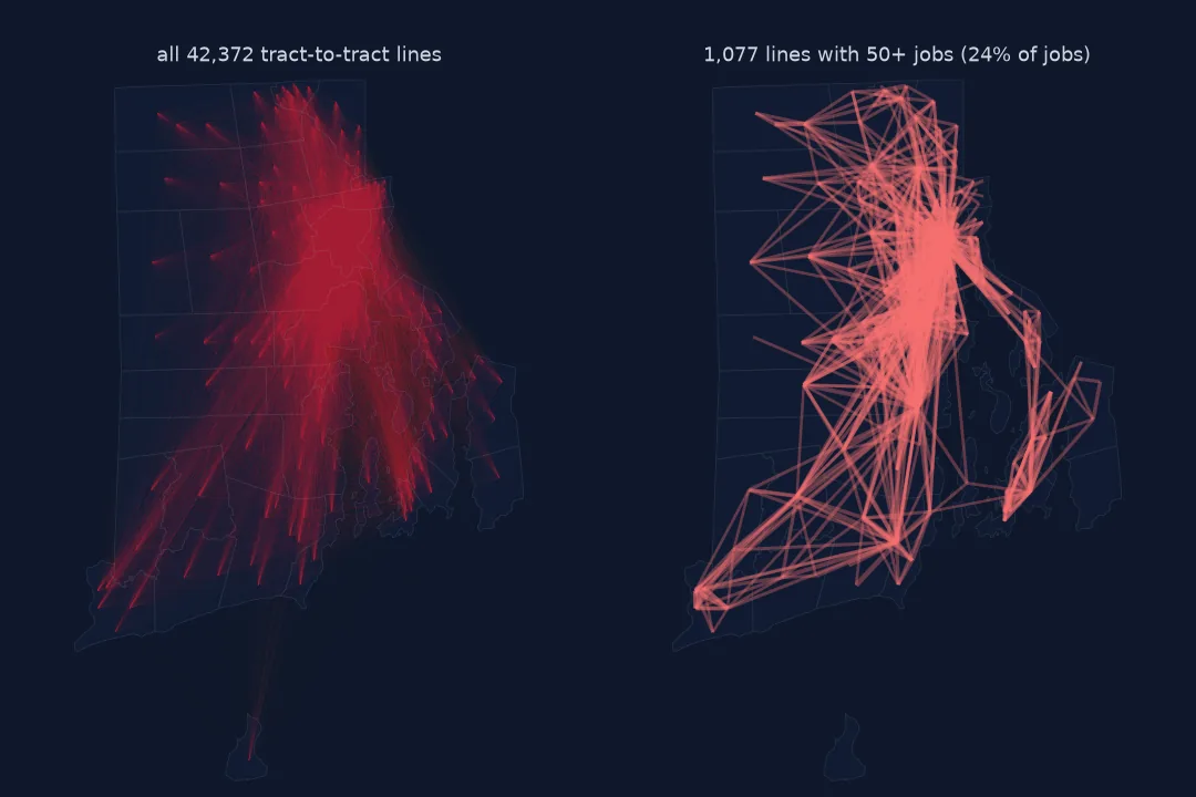
This page builds tract-to-tract commuting desire lines for Rhode Island from LODES, with lines starting at job-weighted tract centres, and keeps the ones that carry most of the commuting.

Quick answer

Aggregate the OD table to zones, give each zone a point, and make one LineString per pair:

pairs = od.groupby(["h_tract", "w_tract"], as_index=False).S000.sum().rename(columns={"S000": "jobs"})
pairs = pairs[pairs.h_tract != pairs.w_tract]
lines = gpd.GeoDataFrame(pairs, geometry=[LineString([PT[h], PT[w]]) for h, w in zip(pairs.h_tract, pairs.w_tract)],
                         crs=3438)
lines["km"] = lines.length * 0.3048 / 1000                                  # EPSG:3438 is in US survey feet
lines.to_file("data/desire_lines.gpkg", layer="tract_commutes")
print(f"{len(lines):,} desire lines, {lines.jobs.sum():,} jobs; median length {lines.km.median():.1f} km")

42,372 desire lines, 360,704 jobs; median length 17.6 km

Two maps of Rhode Island: on the left all 42,372 tract-to-tract commuting desire lines drawn faintly form a dense red mass centred on Providence; on the right the 1,077 lines with at least 50 jobs form a network of corridors converging on Providence, with branches along the coast to Newport and Westerly. — All desire lines against the 1,077 that carry 50 or more jobs each. The filtered map shows the corridors but covers only 24% of commuting between tracts.

Choose the zone point, keep what matters, measure the lines

1. Choose the zone point

A desire line starts at a point, not an area. The polygon centroid can fall in a lake or an empty corner. A better point is the centre of where the people are: the average of the block points, weighted by jobs. Compare the two for each tract:

shift_km = np.array([np.hypot(PT[t][0] - CEN[t][0], PT[t][1] - CEN[t][1]) for t in PT if t in CEN]) * 0.3048 / 1000
print(f"job-weighted point vs polygon centroid: median {np.median(shift_km):.2f} km apart, 90th percentile {np.percentile(shift_km, 90):.1f} km, "
      f"max {shift_km.max():.1f} km")

job-weighted point vs polygon centroid: median 0.24 km apart, 90th percentile 0.8 km, max 4.3 km

2. Keep the lines that matter

Most tract pairs hold a handful of jobs. Rank the lines and see how many it takes to carry the commuting:

s = lines.jobs.sort_values(ascending=False)
share = s.cumsum() / s.sum()
for n in (100, 500, 2000):
    print(f"top {n:>5,} lines: {share.iloc[n - 1]:.0%} of commuting between tracts")
print(f"lines with 50+ jobs: {(lines.jobs >= 50).sum():,} ({lines.loc[lines.jobs >= 50, 'jobs'].sum() / lines.jobs.sum():.0%} of jobs)")

top   100 lines: 5% of commuting between tracts
top   500 lines: 15% of commuting between tracts
top 2,000 lines: 35% of commuting between tracts
lines with 50+ jobs: 1,077 (24% of jobs)

At tract level, commuting is spread very thin. The 500 largest lines carry only 15% of it, and even the 1,077 lines with 50 or more jobs carry under a quarter. A desire-line map at this scale shows the main corridors, not the whole pattern. For that, aggregate to larger zones or summarise the lines by direction and distance.

3. Measure them like any line layer

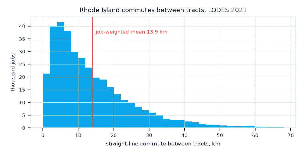
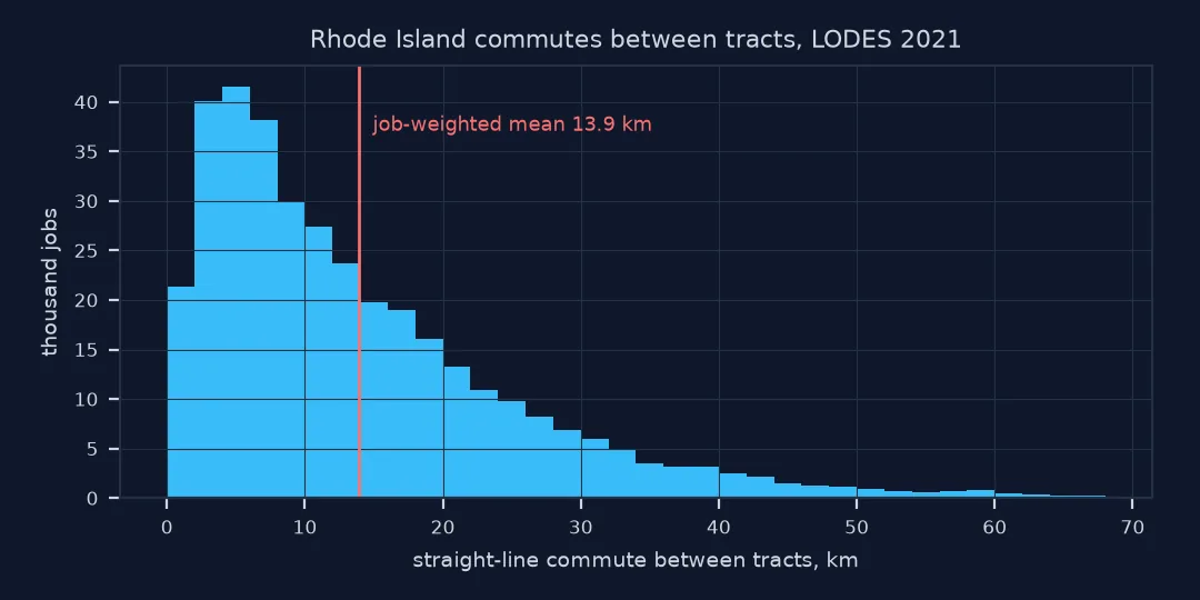
Desire lines are geometry, so lengths, intersections and buffers work directly. How far do people commute in a straight line, and how many desire lines cross Providence's city limits?

w = np.average(lines.km, weights=lines.jobs)
prov = TOWNS.loc[TOWNS.NAME == "Providence"].geometry.iloc[0]
into = lines[lines.intersects(prov)]
print(f"job-weighted mean straight-line commute: {w:.1f} km; {(lines.km < 5).mean():.0%} of lines are shorter than 5 km")
print(f"lines touching Providence: {len(into):,} carrying {into.jobs.sum():,} jobs ({into.jobs.sum() / lines.jobs.sum():.0%})")

job-weighted mean straight-line commute: 13.9 km; 11% of lines are shorter than 5 km
lines touching Providence: 22,164 carrying 161,772 jobs (45%)

Histogram of straight-line commute lengths between tracts weighted by jobs: most commutes are 2 to 10 km, with a long tail to 60 km and a job-weighted mean of 13.9 km. — Straight-line commute lengths between tracts. The road distance is longer; the straight line is a lower bound.

Reading the layer back and filtering it

The data used on this page

LODES version 8 for Rhode Island, 2021 (main, all jobs) and its block crosswalk, which gives each block an internal point and its tract; tract and town outlines from the 2023 cartographic boundary files, projected to Rhode Island State Plane (EPSG:3438, US feet).

from pathlib import Path

import geopandas as gpd
import matplotlib
matplotlib.use("Agg")
import matplotlib.pyplot as plt
import numpy as np
import pandas as pd
import requests
from shapely.geometry import LineString

Path("data").mkdir(exist_ok=True)
L = "https://lehd.ces.census.gov/data/lodes/LODES8/ri/"
G = "https://www2.census.gov/geo/tiger/GENZ2023/shp/"
SRC = {"ri_od_main_JT00_2021.csv.gz": L + "od/ri_od_main_JT00_2021.csv.gz", "ri_xwalk.csv.gz": L + "ri_xwalk.csv.gz",
       "cb_2023_44_tract_500k.zip": G + "cb_2023_44_tract_500k.zip", "cb_2023_44_cousub_500k.zip": G + "cb_2023_44_cousub_500k.zip"}
for name, url in SRC.items():
    if not Path("data", name).exists():
        Path("data", name).write_bytes(requests.get(url, timeout=600).content)
xw = pd.read_csv("data/ri_xwalk.csv.gz", dtype=str, usecols=["tabblk2020", "trct", "blklatdd", "blklondd"]).set_index("tabblk2020")
od = pd.read_csv("data/ri_od_main_JT00_2021.csv.gz", dtype={"w_geocode": str, "h_geocode": str})
od["h_tract"], od["w_tract"] = od.h_geocode.map(xw.trct), od.w_geocode.map(xw.trct)
blk = gpd.GeoSeries(gpd.points_from_xy(xw.blklondd.astype(float), xw.blklatdd.astype(float)), index=xw.index, crs=4326).to_crs(3438)
hjobs = od.groupby("h_geocode").S000.sum()                                   # weight block points by resident workers
wt = pd.DataFrame({"x": blk.x, "y": blk.y, "t": xw.trct, "w": hjobs.reindex(xw.index).fillna(0)})
wt = wt[wt.w > 0]
PT = {t: (np.average(g.x, weights=g.w), np.average(g.y, weights=g.w)) for t, g in wt.groupby("t")}
tracts = gpd.read_file("data/cb_2023_44_tract_500k.zip").to_crs(3438)
CEN = {g: (p.x, p.y) for g, p in zip(tracts.GEOID, tracts.centroid)}
TOWNS = gpd.read_file("data/cb_2023_44_cousub_500k.zip").to_crs(3438)
print(f"{len(PT)} tracts with resident workers; {len(tracts)} tract outlines")

247 tracts with resident workers; 247 tract outlines

Example 1: read the layer back and filter it

back = gpd.read_file("data/desire_lines.gpkg", layer="tract_commutes")
major = back[back.jobs >= 50].sort_values("jobs", ascending=False)
print(f"{len(back):,} lines read back; {len(major):,} with 50 or more jobs; longest of those {major.km.max():.1f} km")

42,372 lines read back; 1,077 with 50 or more jobs; longest of those 42.2 km

Desire lines are deliberately unrealistic

Desire lines are deliberately unrealistic. Nobody drives in a straight line from home to work, and that is the point: the line shows what people want before the network constrains it. A corridor where many desire lines run parallel but no direct road or transit route exists is a candidate for one. Because the lines are a normal vector layer, all of GIS applies. They can be intersected with a city boundary, buffered along a proposed route, or summed by direction.

At tract level commuting is spread thin; any map shows a minority of it.

Two choices shape the result more than any styling. The zone point decides where every line starts. In Rhode Island the job-weighted point is usually within a few hundred metres of the polygon centroid but up to 4.3 km away in large rural tracts. The filter decides what the reader sees. Most lines carry a few jobs each, and a map of all 42,372 is a grey haze. The largest show the corridors, but at tract level they are a minority of the trips, so say what share the map covers.

Units, intrazonal trips and routing

Desire line problems and fixes.

Units: Rhode Island State Plane (EPSG:3438) is in US survey feet; convert before quoting kilometres.
Intrazonal trips have no desire line; report them separately rather than dropping them silently.
Zone size changes line length: larger zones mean more trips are intrazonal and the remaining lines are longer.
Direction: a home → work line and a work → home line between the same tracts are separate rows; merge them if direction does not matter.
Routing: to estimate network distance, route each line's endpoints on a street network; the straight line is a lower bound.

Internal links

How to map commuting flows from LODES — the town-level version
How to make a flow map in Python — styling flows for a map

FAQ

What is a desire line?

A straight line from the origin to the destination of a trip or group of trips, ignoring the route actually taken. It shows travel demand independently of the network.

How do I create desire lines in Python?

Aggregate trips to zone pairs, give each zone a point, and build a shapely.LineString for each pair in a GeoDataFrame with the trip count as an attribute.

Should desire lines start at zone centroids?

A population- or job-weighted point is better than the polygon centroid, especially for large rural zones whose centroid may be far from where people live.

How many desire lines should I map?

Rank the lines and report the share of trips your selection covers. With small zones, as here, even a thousand lines carry under a quarter of the trips; larger zones concentrate the volume.