How to Build and Read an Origin–Destination Matrix in Python

On this page

Problem statement

An origin–destination (OD) matrix is the table behind every flow map: one row per origin, one column per destination, and the number of trips, moves or commuters in each cell. A flow map shows a few dozen of its cells. The matrix holds all of them, and some questions are easier to answer from the matrix than from any map. How much does each place send and attract? How self-contained is it? Which flows are mostly one-way? Building one from a long table is a pivot. Reading it well depends on the order of rows and columns, a log colour scale, and knowing what the diagonal means.

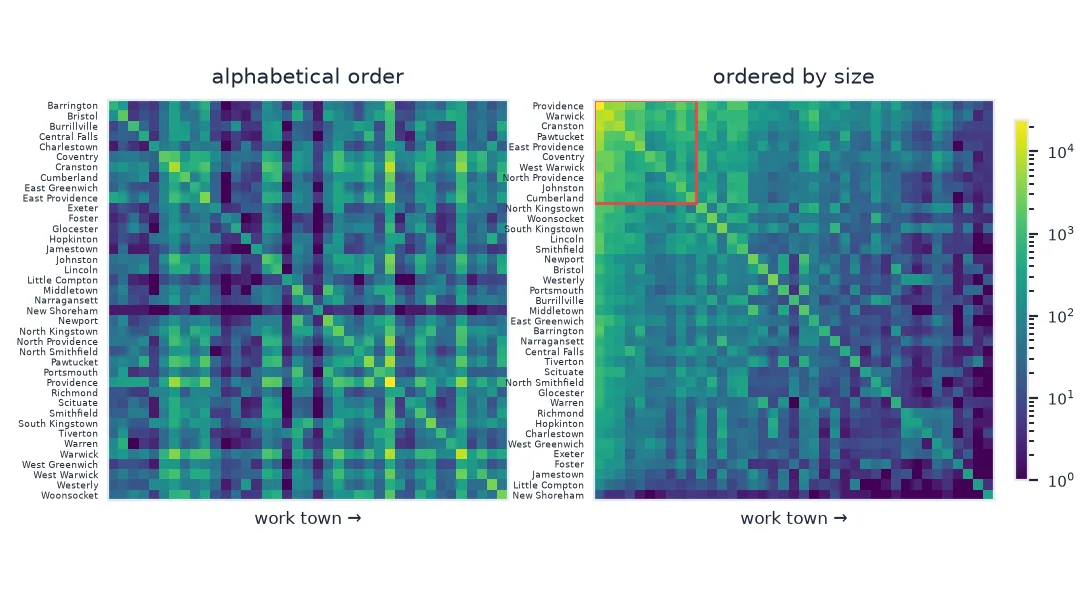
This page builds the 39 × 39 town matrix of Rhode Island commuting from LODES and reads it four ways.

Quick answer

Pivot the long table of flows into a square matrix with the same order for rows and columns, fill missing pairs with zero, and plot it on a log scale:

order = TOWNS.sort_values("pop", ascending=False).GEOID.tolist()          # biggest towns first
M = tt.pivot(index="home", columns="work", values="jobs").reindex(index=order, columns=order).fillna(0)
fig, ax = plt.subplots(figsize=(8, 7))
im = ax.imshow(M + 1, norm=LogNorm(1, M.to_numpy().max()), cmap="viridis")
ax.set_xticks(range(len(order)), [NAME[g] for g in order], rotation=90, fontsize=6)
ax.set_yticks(range(len(order)), [NAME[g] for g in order], fontsize=6)
fig.colorbar(im, label="jobs (log)"); fig.savefig("data/od_matrix.png", dpi=150, bbox_inches="tight")
print(f"{M.shape[0]} x {M.shape[1]} matrix, {(M > 0).to_numpy().mean():.0%} of cells non-zero, total {M.to_numpy().sum():,.0f} jobs")

39 x 39 matrix, 96% of cells non-zero, total 380,586 jobs

Two heatmaps of the same 39 by 39 Rhode Island commuting matrix on a log colour scale: in alphabetical order the bright cells are scattered across the grid; ordered by size, bright cells gather in the top-left corner around Providence, Warwick and Cranston, outlined in red, and along the diagonal. — The same matrix in two orders. Sorted by size, 47% of all jobs fall in the top-left 10 × 10 block; in alphabetical order, 9%.

Margins, diagonal, net and two-way flow, ordering

1. Read the margins

Row sums are what each origin sends (resident workers); column sums are what each destination attracts (jobs). Their ratio says whether a town is a net importer or exporter of workers:

sent, attracted = M.sum(axis=1), M.sum(axis=0)
ratio = (attracted / sent).rename(NAME)
print("most jobs per resident worker:", ", ".join(f"{t} {v:.2f}" for t, v in ratio.nlargest(3).items()))
print("fewest:                        ", ", ".join(f"{t} {v:.2f}" for t, v in ratio.nsmallest(3).items()))

most jobs per resident worker: Providence 1.68, Middletown 1.61, Smithfield 1.49
fewest:                         Foster 0.19, Scituate 0.30, Hopkinton 0.32

2. Read the diagonal

The diagonal is people who live and work in the same town. As a share of each row it measures self-containment, as a share of each column how much a town's jobs are filled locally:

d = pd.Series(np.diag(M), index=M.index)
contain = (d / sent).rename(NAME)
local = (d / attracted).rename(NAME)
print(f"self-containment (live and work in town): median {contain.median():.0%}, Providence {contain['Providence']:.0%}")
print(f"jobs filled by residents: median {local.median():.0%}, Providence {local['Providence']:.0%}")

self-containment (live and work in town): median 18%, Providence 45%
jobs filled by residents: median 27%, Providence 27%

3. Split each pair into net and two-way flow

For any pair of towns, the flow one way and the flow back can be split into a symmetric part (the smaller of the two) and a net part (the difference). A matrix whose off-diagonal flows are mostly symmetric describes exchange; one dominated by the net part describes a one-way pull:

A = M.to_numpy(copy=True); np.fill_diagonal(A, 0)
sym = np.minimum(A, A.T); net = A - sym
print(f"off-diagonal flow: {A.sum():,.0f}; two-way part {sym.sum():,.0f} ({sym.sum() / A.sum():.0%}), one-way part {net.sum():,.0f}")
i, j = np.unravel_index(net.argmax(), net.shape)
print(f"largest one-way excess: {NAME[order[i]]} -> {NAME[order[j]]}, {net[i, j]:,.0f} more than flow back ({A[j, i]:,.0f})")

off-diagonal flow: 292,363; two-way part 196,352 (67%), one-way part 96,011
largest one-way excess: Cranston -> Providence, 3,696 more than flow back (5,601)

In Rhode Island two thirds of the commuting between towns is matched by commuting back the other way. The one-way part is still large, and its biggest single piece is the extra flow from Cranston into Providence.

Two thirds of commuting between Rhode Island towns is exchange.

4. Order rows and columns deliberately

The same matrix looks random or structured depending on the order. Alphabetical order scatters the strong cells; ordering by size puts the big towns and their large flows in the top-left corner. Compare how much of the flow lands in the top-left 10 × 10 block:

def corner_share(order, k=10):
    m = tt.pivot(index="home", columns="work", values="jobs").reindex(index=order, columns=order).fillna(0).to_numpy()
    return m[:k, :k].sum() / m.sum()

alpha = sorted(order, key=lambda g: NAME[g])
print(f"jobs in the top-left 10 x 10: by population {corner_share(order):.0%}, alphabetical {corner_share(alpha):.0%}")

jobs in the top-left 10 x 10: by population 47%, alphabetical 9%

The Rhode Island matrix as a table

The data used on this page

LODES version 8, Rhode Island 2021: the main OD file for all jobs and the block crosswalk; town outlines from the 2023 cartographic boundary files. Town population for ordering is the number of LODES resident workers.

from pathlib import Path

import geopandas as gpd
import matplotlib
matplotlib.use("Agg")
import matplotlib.pyplot as plt
import numpy as np
import pandas as pd
import requests
from matplotlib.colors import LogNorm

Path("data").mkdir(exist_ok=True)
L = "https://lehd.ces.census.gov/data/lodes/LODES8/ri/"
SRC = {"ri_od_main_JT00_2021.csv.gz": L + "od/ri_od_main_JT00_2021.csv.gz", "ri_xwalk.csv.gz": L + "ri_xwalk.csv.gz",
       "cb_2023_44_cousub_500k.zip": "https://www2.census.gov/geo/tiger/GENZ2023/shp/cb_2023_44_cousub_500k.zip"}
for name, url in SRC.items():
    if not Path("data", name).exists():
        Path("data", name).write_bytes(requests.get(url, timeout=600).content)
xw = pd.read_csv("data/ri_xwalk.csv.gz", dtype=str, usecols=["tabblk2020", "ctycsub"]).set_index("tabblk2020").ctycsub
od = pd.read_csv("data/ri_od_main_JT00_2021.csv.gz", dtype={"w_geocode": str, "h_geocode": str})
tt = (od.assign(home=od.h_geocode.map(xw), work=od.w_geocode.map(xw))
        .groupby(["home", "work"], as_index=False).S000.sum().rename(columns={"S000": "jobs"}))
TOWNS = gpd.read_file("data/cb_2023_44_cousub_500k.zip")
TOWNS = TOWNS[TOWNS.ALAND > 0].assign(pop=lambda d: d.GEOID.map(tt.groupby("home").jobs.sum()))
NAME = dict(zip(TOWNS.GEOID, TOWNS.NAME))
print(f"{len(tt):,} town pairs, {tt.jobs.sum():,} jobs, {len(TOWNS)} towns")

1,466 town pairs, 380,586 jobs, 39 towns

Example 1: the matrix as a table

small = M.rename(index=NAME, columns=NAME).iloc[:5, :5].astype(int)
print(small.to_string())

work             Providence  Warwick  Cranston  Pawtucket  East Providence
home                                                                      
Providence            24131     4631      5601       2534             2434
Warwick                7710     9808      3753        998             1443
Cranston               9297     4528      6702       1041             1441
Pawtucket              6132     1782      1508       4399             1787
East Providence        5145     1346      1066        959             3682

The matrix is the record; a map is a selection

The matrix is the complete record; a flow map is a selection from it. Reading the matrix first tells you what to put on the map. The margins say which places matter, the diagonal how much stays local, and the symmetric split whether flows are exchange or pull. A log colour scale is not optional. Cell values range from one job to tens of thousands, and on a linear scale everything but the diagonal disappears.

Four readings of one matrix.

Ordering is the other decision that changes what the matrix shows. Rows and columns must use the same order, or the diagonal stops being the diagonal. Within that rule, sorting by size, by geography or by a clustering of the flows each brings out different structure. Here ordering by size gathers the Providence-centred core into one corner.

Sparse storage, missing pairs and row normalising

OD matrix problems and fixes.

Sparse matrices: with hundreds of zones, store the long table or a scipy.sparse matrix; a dense pivot of tracts is mostly zeros.
Missing pairs are zero flows only if the source reports all non-zero pairs; check the documentation before filling with zero.
Same order on both axes: use one list for reindex(index=..., columns=...).
Asymmetric definitions: migration matrices (from, to) and commuting matrices (home, work) both have direction; say which axis is which in the labels.
Normalising rows (row shares) answers "where do people from here go"; normalising columns answers "where do workers here come from".

Internal links

How to map commuting flows from LODES — the flows behind this matrix
Origin–destination data explained — what an OD table is and is not

FAQ

How do I make an OD matrix in pandas?

Pivot a long table of (origin, destination, count) with pivot or pivot_table, reindex rows and columns to the same order, and fill missing pairs with zero.

How should I visualise an origin–destination matrix?

As a heatmap with a log colour scale, rows and columns in the same deliberate order (by size, geography or clusters).

What does the diagonal of an OD matrix mean?

Flows that start and end in the same zone: people who work in their home town, or moves within a county.

What is self-containment?

The share of a zone's residents who also work (or stay) in that zone: the diagonal divided by the row total.