How to Read the US Wind Turbine Database in Python

Problem statement

The US Geological Survey keeps a list of every utility-scale wind turbine in the United States, each placed on aerial imagery to within about ten metres: the US Wind Turbine Database. One CSV row is one turbine, with its project, its maker and model, its capacity, hub height and rotor size, and its coordinates. It is the file behind most maps of American wind power. Read naively, it loses the leading zeros of its county codes, mixes kilowatts with megawatts, and leaves a few thousand turbines without specifications. This page reads version 9.1, published on 28 September 2026, and shows what is in it.

Quick answer

Read the CSV with the county code as text, and sum the turbine capacity column, which is in kilowatts:

wt = pd.read_csv(Z.open("uswtdb_V9_1_20260928.csv"), dtype={"t_fips": str})
print(f"{len(wt):,} turbines, {wt.p_name.nunique():,} project names, {wt.t_cap.sum() / 1e6:.1f} GW of rated capacity")
print(wt.iloc[0][["p_name", "t_state", "p_year", "t_manu", "t_model", "t_cap", "t_hh", "t_rd", "xlong", "ylat"]].to_string())

77,839 turbines, 1,805 project names, 159.6 GW of rated capacity
p_name     25 Mile Creek
t_state               OK
p_year            2022.0
t_manu            Vestas
t_model         V150-4.2
t_cap             4200.0
t_hh               105.0
t_rd               150.0
xlong         -99.756958
ylat           36.491249

Version 9.1 lists 77,839 turbines under 1,805 project names, with 159.6 GW of rated capacity between them. The first row is a 4.2 MW Vestas V150 at the 25 Mile Creek project in Ellis County, Oklahoma, online in 2022, on a 105 m hub with a 150 m rotor. The coordinates are in NAD83, so the points are created with EPSG:4269.

One row per turbine

1. Three kinds of column

kinds = wt.columns.str.split("_").str[0]
print(kinds.value_counts().to_string())
print([c for c in wt.columns if c.startswith("p_")])

t        17
p         4
faa       2
case      1
usgs      1
eia       1
xlong     1
ylat      1
['p_name', 'p_year', 'p_tnum', 'p_cap']

The prefix says what a column describes. Seventeen t_ columns describe the turbine: its state, county, model, capacity, sizes, retrofit flag, confidence codes and the imagery it was checked on. Four p_ columns describe the project the turbine belongs to and are repeated on each of its turbines. The rest are identifiers that link to other datasets: case_id is USGS's own stable key, faa_ors and faa_asn lead to the FAA's obstacle records, eia_id to the plant in EIA-860, and usgs_pr_id to the older USGS turbine dataset.

2. Units

print(wt[["t_cap", "p_cap", "t_hh", "t_rd", "t_ttlh"]].describe().loc[["min", "50%", "max"]].round(1).to_string())

       t_cap   p_cap   t_hh   t_rd  t_ttlh
min     50.0     0.0   19.0   13.4    30.5
50%   2000.0   176.9   80.0  101.0   134.1
max  14000.0  1055.6  140.0  222.0   247.5

t_cap is in kilowatts: the median turbine is rated at 2,000 kW, the largest at 14,000 kW. p_cap is in megawatts, for the whole project. The heights and the rotor diameter are in metres, and t_ttlh is the height to the tip of a blade pointing straight up. The two capacity columns differ by a factor of a thousand in unit and describe different things, so they are never added together.

3. What is missing

miss = wt.isna().sum()
print(miss[miss > 0].sort_values().to_string())

t_county        124
t_fips          124
t_state         124
p_year          842
faa_ors        3349
faa_asn        3556
p_cap          3857
t_manu         4866
t_model        4909
eia_id         5051
t_cap          5056
t_rd           5140
t_rsa          5140
t_hh           5450
t_ttlh         5500
t_img_date     6467
usgs_pr_id    41912
t_retro_yr    69130

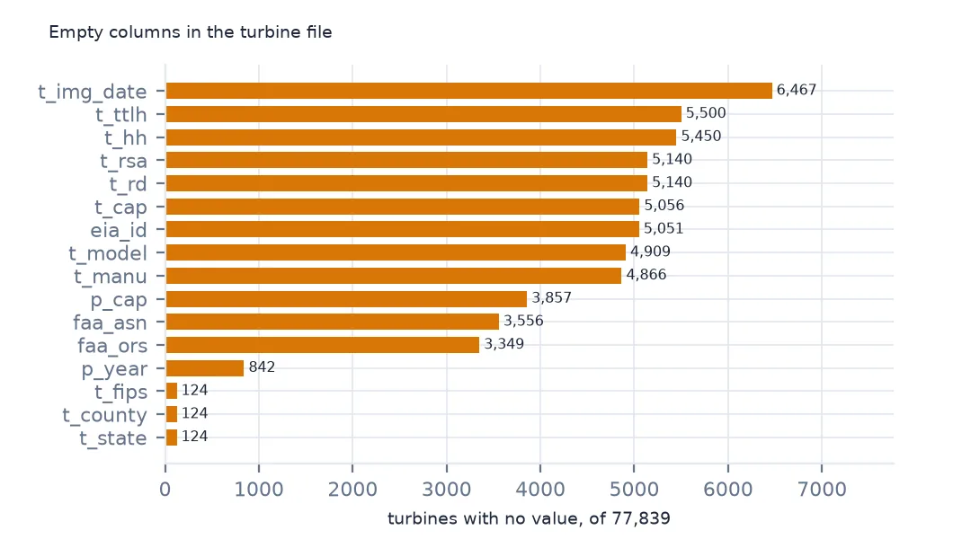
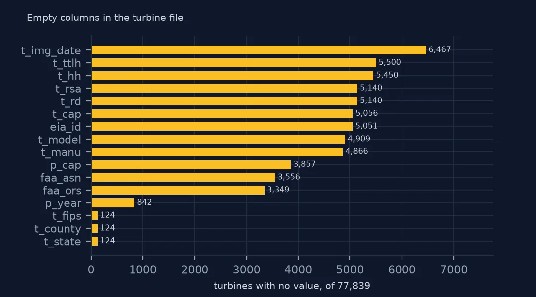
The 124 rows without a state or county are offshore turbines in federal waters. About 5,000 turbines, 6.5% of the file, have no model, capacity or size. They are mostly the newest projects, which USGS has placed on imagery before their specifications are known. t_retro_yr is empty unless the turbine was rebuilt, and usgs_pr_id only exists for turbines that were in the older USGS dataset.

States and a map

The data used on this page

The US Geological Survey's US Wind Turbine Database, version 9.1 of 28 September 2026 (Hoen and others, doi:10.5066/F7TX3DN0), public domain. USGS replaces the file every quarter, so the version used here was saved on this site on 19 October 2026 with its metadata and changelog. With it come the Census Bureau's 2024 county boundaries and the wind table of EIA-860 for 2025.

from pathlib import Path
import zipfile

import geopandas as gpd
import pandas as pd
import requests

Path("data").mkdir(exist_ok=True)
# USGS US Wind Turbine Database v9.1 (28 September 2026) with its metadata and changelog, Census 2024 cartographic
# boundary counties and the EIA-860 2025 wind table. Saved 19 October 2026: USGS replaces the file every quarter.
# Live: https://energy.usgs.gov/uswtdb/assets/data/uswtdbCSV.zip
ARCHIVE = "usgs-uswtdb-v9-1-2026-10-19.zip"
if not Path(f"data/{ARCHIVE}").exists():
    Path(f"data/{ARCHIVE}").write_bytes(requests.get(f"https://data.spatialworkflow.io/{ARCHIVE}", timeout=600).content)
Z = zipfile.ZipFile(f"data/{ARCHIVE}")
wt = pd.read_csv(Z.open("uswtdb_V9_1_20260928.csv"), dtype={"t_fips": str})
Path("data/cb_2024_us_county_20m.zip").write_bytes(Z.read("cb_2024_us_county_20m.zip"))
counties = gpd.read_file("data/cb_2024_us_county_20m.zip")
print(f"US Wind Turbine Database v9.1: {len(wt):,} turbines; counties: {len(counties):,}")

US Wind Turbine Database v9.1: 77,839 turbines; counties: 3,222

Example 1: turbines and capacity by state

st = wt.groupby("t_state").agg(turbines=("case_id", "size"), gw=("t_cap", lambda s: s.sum() / 1e6))
st = st.sort_values("gw", ascending=False)
print(st.head(6).round(1).to_string())
print(f"states and territories with turbines: {len(st)}; top three's share of capacity: {st.gw.head(3).sum() / st.gw.sum():.1%}")

         turbines    gw
t_state                
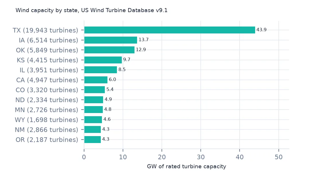
TX          19943  43.9
IA           6514  13.7
OK           5849  12.9
KS           4415   9.7
IL           3951   8.5
CA           4947   6.0
states and territories with turbines: 47; top three's share of capacity: 44.5%

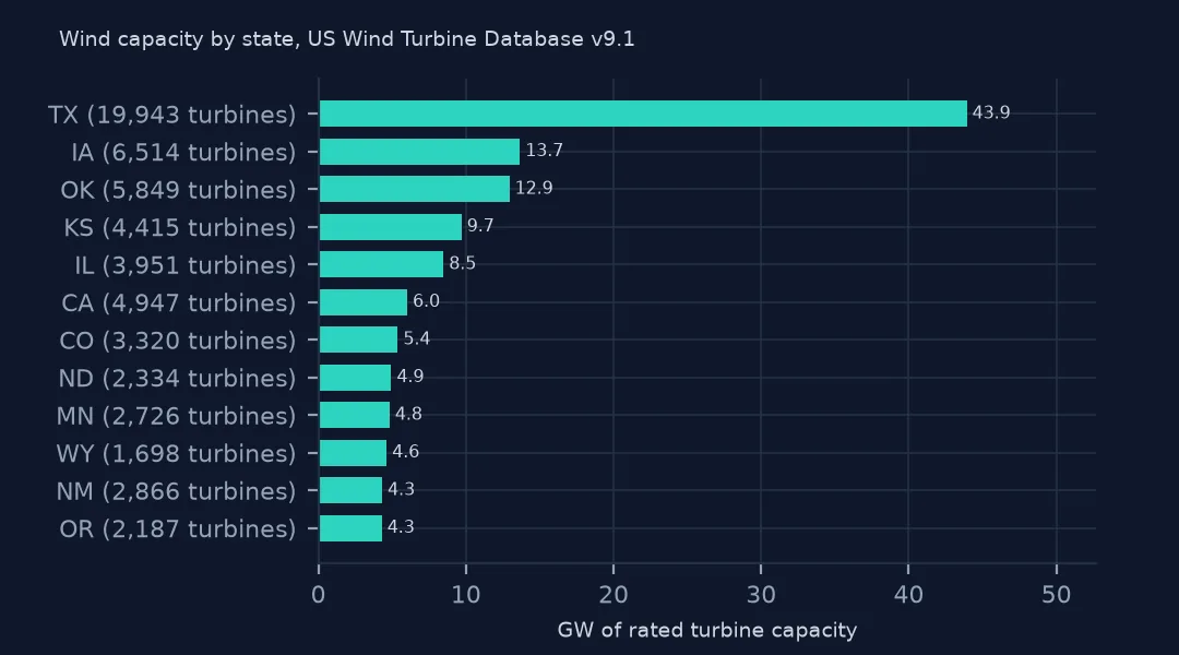
Texas has 19,943 turbines and 43.9 GW, more than the next three states together, and Texas, Iowa and Oklahoma hold 44.5% of the national capacity. California has more turbines than Kansas or Illinois but less capacity: many of its turbines are small machines from the 1980s in the Altamont, Tehachapi and San Gorgonio passes.

Example 2: every turbine on a map

g = gpd.GeoDataFrame(wt, geometry=gpd.points_from_xy(wt.xlong, wt.ylat), crs=4269)
away = ["AK", "HI", "PR", "GU"]
print(g[g.t_state.isin(away)].groupby("t_state").size().to_string())
print("offshore, no state:", g.t_state.isna().sum())
lower48 = g[~g.t_state.isin(away) & g.t_state.notna()].to_crs(5070)
ax = lower48.plot(markersize=0.3, figsize=(10, 6))
ax.set_axis_off()

t_state
AK    144
GU      1
HI    128
PR     63
offshore, no state: 124

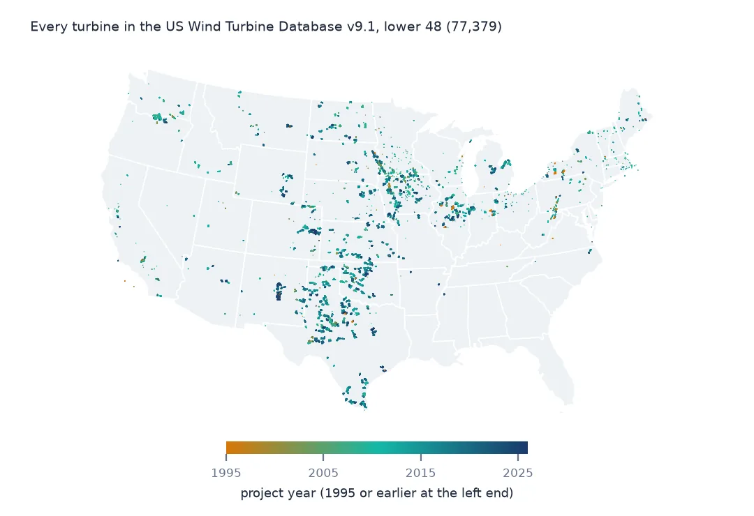
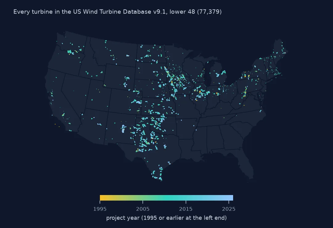
Outside the lower 48 there are 144 turbines in Alaska, 128 in Hawaii, 63 in Puerto Rico and one on Guam. The 124 offshore turbines with no state are left out of the map along with them. Plotted in an equal-area projection, the rest trace the wind belt from the Texas panhandle north through the plains to the Dakotas, with clusters in the Midwest, the Columbia Gorge and California's passes.

Internal links

• Where each record comes from — sources, confidence codes and quarterly versions
• Capacity by county — the county code read as text, then mapped
• Project capacity summed per turbine — why p_cap must not be summed
• Turbines against EIA-860 — the eia_id join
• Offshore turbines — the 124 rows with no state