
How to Measure Wind Turbine Spacing in Rotor Diameters
On this page
Problem statement
Wind farm layouts are described in rotor diameters, not metres: a turbine slows and churns the wind behind it, and how far that wake reaches scales with the size of the rotor. Spacing in metres alone says little, because a 2005 turbine with a 77 m rotor and a 2025 turbine with a 140 m rotor need different gaps. The US Wind Turbine Database has a position and a rotor diameter for almost every turbine, so the spacing that projects actually use can be measured: project the points to metres, find each turbine's nearest neighbour, and divide the distance by the rotor diameter. The same measurement also finds records that sit on top of each other. This page does it for all 77,839 turbines of version 9.1.
Quick answer
Project to an equal-area CRS in metres, query a KD-tree for the two nearest points (the first is the turbine itself), and divide by t_rd:
g = gpd.GeoDataFrame(wt, geometry=gpd.points_from_xy(wt.xlong, wt.ylat), crs=4269).to_crs(5070)
xy = np.c_[g.geometry.x, g.geometry.y]
dist, idx = cKDTree(xy).query(xy, k=2)
g["nn_m"], g["nn_id"] = dist[:, 1], idx[:, 1]
g["nn_d"] = g.nn_m / g.t_rd
print(g.nn_d.describe(percentiles=[0.1, 0.25, 0.5, 0.75, 0.9]).round(2).loc[["count", "10%", "25%", "50%", "75%", "90%"]].to_string())
count 72699.00
10% 2.42
25% 3.02
50% 3.65
75% 4.76
90% 6.51
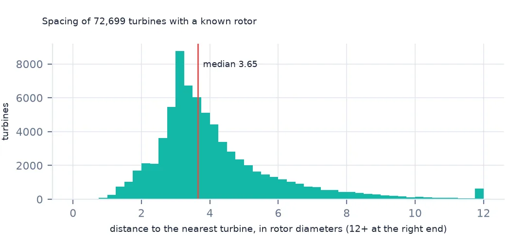
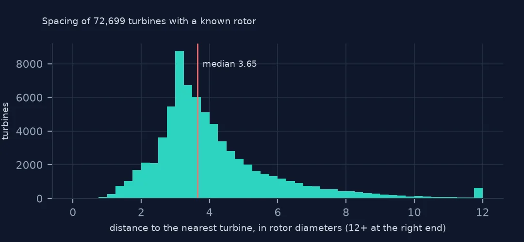
For the 72,699 turbines with a known rotor, the median nearest neighbour stands 3.65 rotor diameters away, and half of all turbines are 3.0 to 4.8 diameters from the next. The projection matters: EPSG:5070 is in metres across the whole lower 48, where distances computed on raw longitude and latitude would be in degrees and shrink towards the north.
Nearest neighbours, checked
1. The nearest turbine is in the same project
same = g.p_name.values == g.p_name.values[g.nn_id]
print(f"nearest neighbour in the same project: {same.mean():.1%}; median spacing {g.nn_m.median():.0f} m")
nearest neighbour in the same project: 97.5%; median spacing 387 m
The nearest turbine is almost always one in the same row: rows are laid out across the prevailing wind with turbines a few diameters apart, and the rows themselves stand further apart. So this measures the spacing within a row.
2. Records on top of each other
close = g[g.nn_m < 10].assign(other=lambda d: g.p_name.values[d.nn_id])
print(f"turbines with another record within 10 m: {len(close)}; within 1 m: {(close.nn_m < 1).sum()}")
print(close[close.p_name != close.other][["p_name", "other", "t_state", "nn_m"]].round(2).head(4).to_string(index=False))
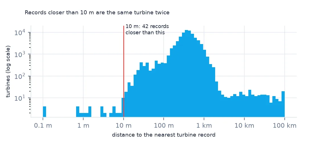
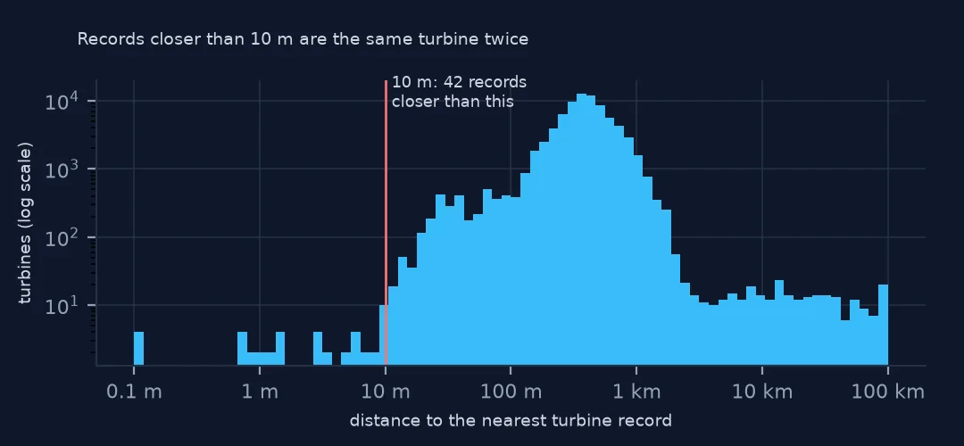
turbines with another record within 10 m: 42; within 1 m: 12
p_name other t_state nn_m
Big Sampson Wind unknown Crockett County TX 0.88
Chickasaw County Wind Energy Center unknown Chickasaw County IA 3.07
Clearwater Clearwater Energy Project 1A MT 0.99
Clearwater Energy Project 1A Clearwater MT 0.99
USGS places each turbine on aerial imagery within about 10 m of its tower, and no two towers stand that close. Points under 10 m apart are the same turbine recorded twice, often under two project names. Version 9.1 itself removed 53 duplicates, and these are ones it has not found yet.
Spacing over time
The data used on this page
The US Geological Survey's US Wind Turbine Database, version 9.1 of 28 September 2026 (Hoen and others, doi:10.5066/F7TX3DN0), public domain, saved on this site on 19 October 2026 because USGS replaces the file every quarter.
from pathlib import Path
import zipfile

import geopandas as gpd
import numpy as np
import pandas as pd
import requests
from scipy.spatial import cKDTree

Path("data").mkdir(exist_ok=True)
# USGS US Wind Turbine Database v9.1 (28 September 2026) with its metadata and changelog, Census 2024 cartographic
# boundary counties and the EIA-860 2025 wind table. Saved 19 October 2026: USGS replaces the file every quarter.
# Live: https://energy.usgs.gov/uswtdb/assets/data/uswtdbCSV.zip
ARCHIVE = "usgs-uswtdb-v9-1-2026-10-19.zip"
if not Path(f"data/{ARCHIVE}").exists():
    Path(f"data/{ARCHIVE}").write_bytes(requests.get(f"https://data.spatialworkflow.io/{ARCHIVE}", timeout=600).content)
Z = zipfile.ZipFile(f"data/{ARCHIVE}")
wt = pd.read_csv(Z.open("uswtdb_V9_1_20260928.csv"), dtype={"t_fips": str})
print(f"US Wind Turbine Database v9.1: {len(wt):,} turbines; rotor diameter known for {wt.t_rd.notna().sum():,}")
US Wind Turbine Database v9.1: 77,839 turbines; rotor diameter known for 72,699
Example 1: by five-year period
on = g[(g.t_offshore == 0) & (g.t_retrofit == 0) & (g.p_year >= 2000)]
period = (on.p_year // 5 * 5).astype(int)
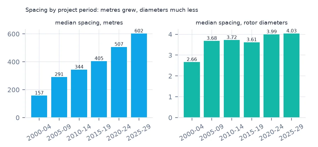
print(on.groupby(period).agg(turbines=("nn_m", "size"), metres=("nn_m", "median"), rotor_m=("t_rd", "median"), diameters=("nn_d", "median")).round(2).to_string())
turbines metres rotor_m diameters
p_year
2000 1939 157.10 52.0 2.66
2005 11682 290.78 77.0 3.68
2010 13927 343.92 90.0 3.72
2015 17753 404.74 110.0 3.61
2020 16459 506.64 127.0 3.99
2025 3739 602.20 140.0 4.03
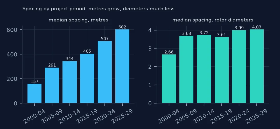
In metres, the median gap almost quadrupled between the early 2000s and the late 2020s, and most of that growth is the rotor: measured in diameters, spacing widened from about 2.7 to about 4.
Example 2: offshore
off = g[g.t_offshore == 1]
print(f"offshore: {len(off)} turbines, median spacing {off.nn_m.median():,.0f} m = {off.nn_d.median():.1f} rotor diameters")
offshore: 129 turbines, median spacing 1,837 m = 8.6 rotor diameters
The offshore projects are laid out on a grid of roughly one nautical mile in every direction, about 1,850 m, which with rotors of 150 to 220 m is more than twice the onshore spacing in diameters.
Internal links
- Turbine sizes by year — the rotors the spacing is measured in
- Offshore turbines — the grid layouts of Example 2
- Nearest-neighbour joins — nearest features, the method on its own
- Reading the database — positions and their accuracy